VSDEL user guide
Everything in the tool, explained with pictures. Type in the search box (or press /) to filter every section live; inside the app, each diagram view's ⓘ Guide button carries the same guidance in place.
Getting started
VSDEL runs in the browser at app.vsdel.com. Sign up with your email — no invitation needed. On first sign-in you either create a team (you become its admin, with a workspace all your own), join with an invite code a team admin gave you, or seed a demo team to explore a ready-made satellite model.
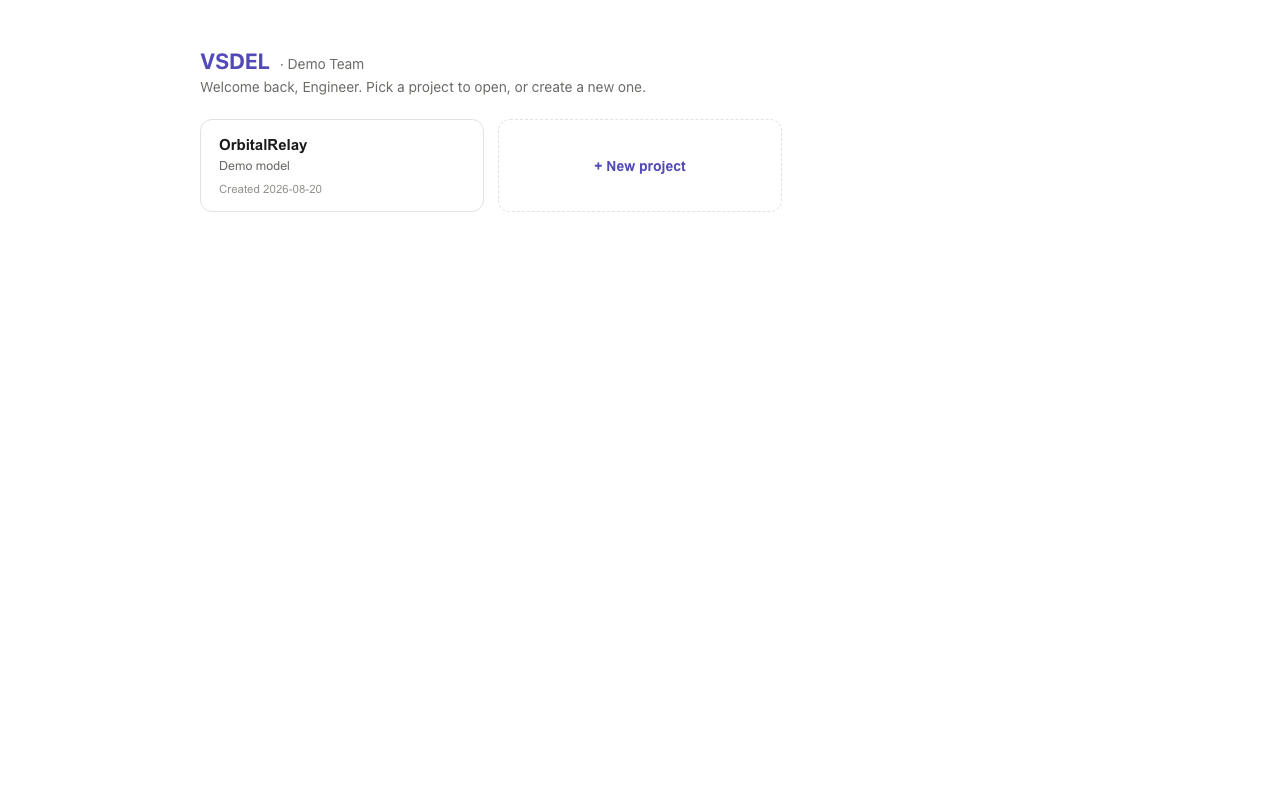
Once you're on a team, the project picker lists your team's projects. + New project offers three starts: Blank, the MBSE skeleton (Structure / Behavior / Requirements / Use cases packages ready to fill), or start from a sample: the OrbitalRelay satellite (a compact model across every lens), the Notation Gallery ground station — every diagram kind and notation in one model, ideal for learning what each symbol means — or the Constellation mission — relay satellites, a patrol aircraft on a waypoint route, ground stations, sensors, coverage requirements and a baseline scenario, ready to run in the Mission scenario analysis lens.
Orientation: finding your way around
The workspace has four standing regions:
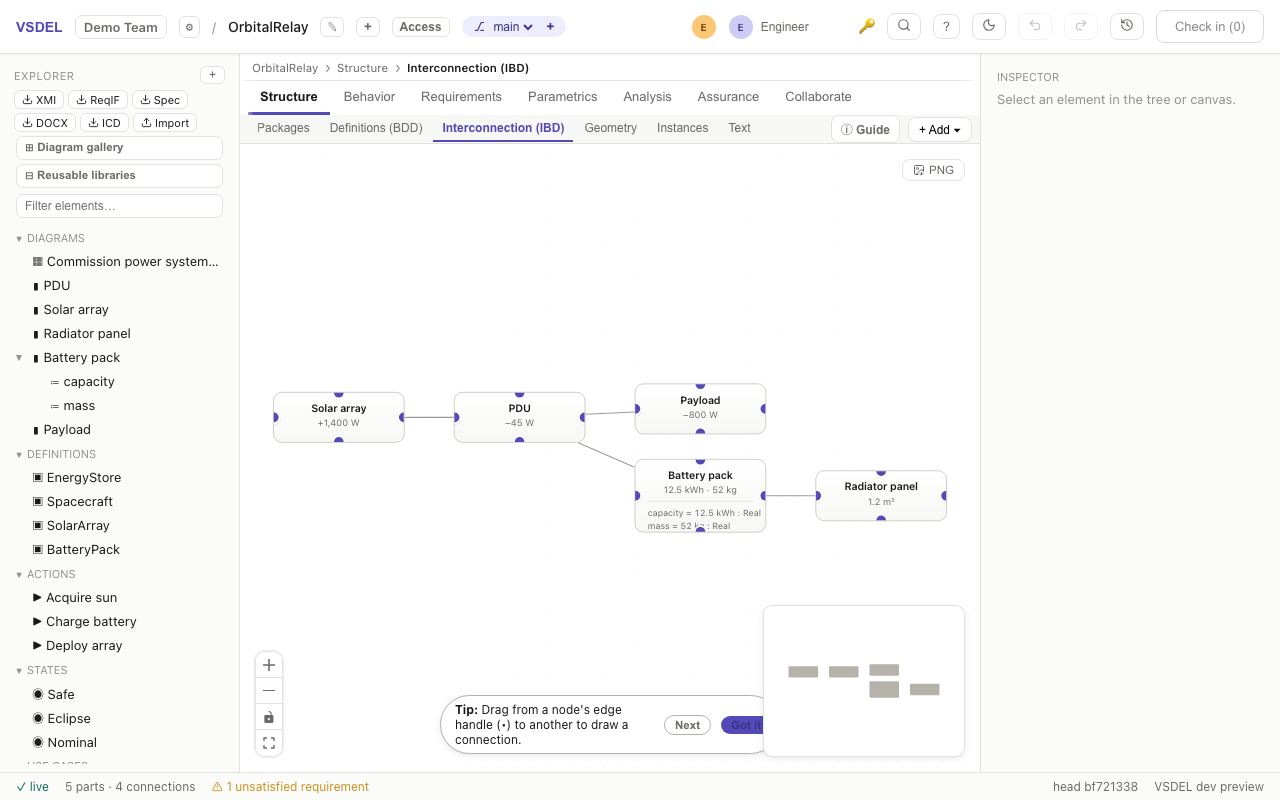
- Explorer tree (left) — every element, grouped by kind and nested by ownership. Click to select, double-click a diagram to open it, drag an element onto the canvas to add it to the open diagram.
- Pillar tabs & views (top) — Structure, Behavior, Requirements, Parametrics, Analysis, Assurance, Collaborate. Each pillar holds views; every view is a live lens over the same model, so an edit in one view shows up in all of them.
- Canvas (center) — the active diagram. A named diagram shows its SysML frame (
bdd [package] Structure); the view tab without a diagram shows the overview canvas of everything the view can render. - Inspector (right) — every property of the selected element, plus contextual actions (add features, create instances, decompose, trace links).
Getting around fast
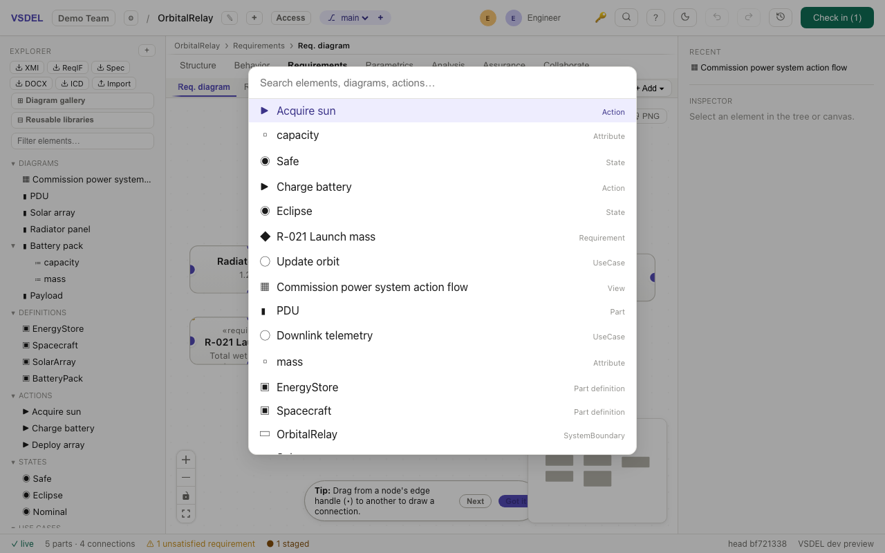
Press ⌘K/Ctrl+K for the command palette — jump to any element, diagram, or view by name. Press ? for the keyboard cheatsheet. The Diagram gallery (top of the tree) shows schematic thumbnails of every named diagram. New to the notation? ⌘K → Notation reference opens a built-in SysML v2 cheat-sheet that draws every glyph and line with the same engine as your diagrams.
The model is a repository
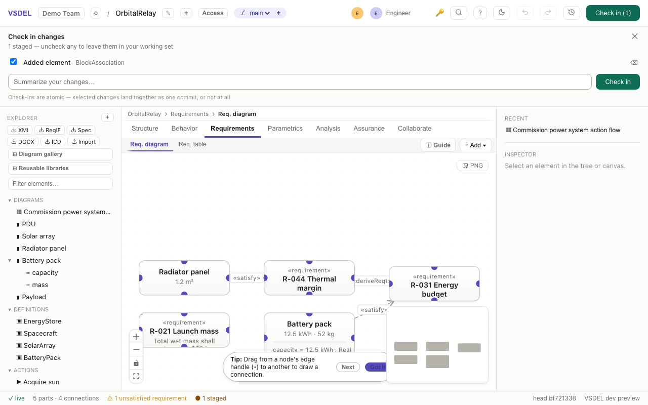
Every element — parts, requirements, states, even diagrams — is a versioned element. Edits stage into your personal working set as you make them (the N staged counter, bottom bar). Nothing is shared until you check in.
- Check in (top right) opens the drawer: review each staged change, uncheck any to leave for later, discard what you don't want (Discard checked (N) clears a whole set), write a summary, commit. Commits are atomic.
- Branches — spin a sandbox for a trade study from the branch picker in the top bar; merge back with conflict resolution.
- Reviews — open a review on a branch and let a colleague walk the diff and approve (Collaborate pillar).
- History — any commit can be diffed, tagged as a baseline, or exported as a document (⟲ icon, top bar).
- Undo/redo (⌘Z) work on your staged edits; check-out locks (inspector) reserve an element when you need pessimistic safety.
Definitions (BDD) — blocks and types
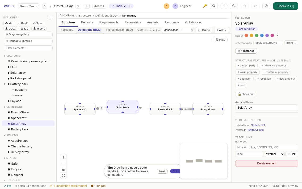
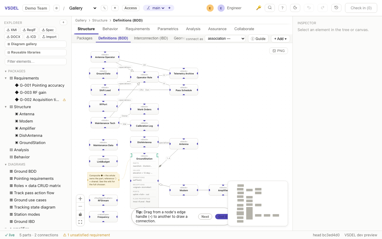
The Block Definition Diagram defines your system's types: blocks, value types, interfaces, constraint blocks. A block's own structure renders as compartments — parts, references, values, constraints, operations, receptions, flow properties, and ports — added from the inspector's quick-add grid or the block's right-click menu.
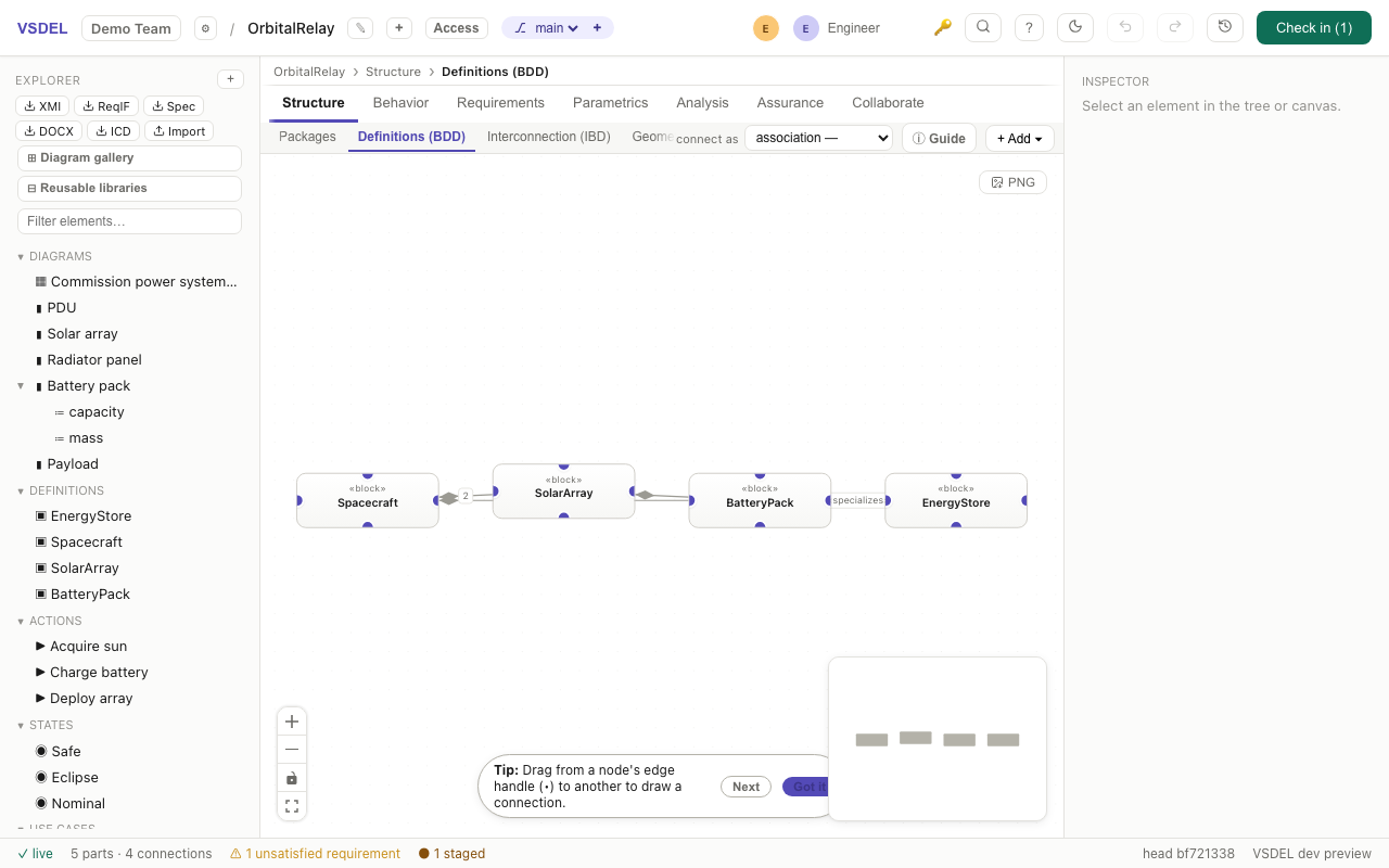
Choosing the right connection
| Draw | Meaning |
|---|---|
| association | a structural relationship without ownership; the plain line. Refine it in the inspector. |
| composite ◆ | the source owns the target as a part (whole–part). The filled diamond renders at the whole end — draw from the owner. endLabel holds multiplicity ("2", "1..4"). |
| reference ◇ | the source uses the target without owning it (shared aggregation) — hollow diamond. |
| generalization | the source is a specialized kind of the target; hollow triangle points at the general. |
| dependency | a weak "source needs target" — dashed with an open arrow. |
| usage → definition | typing: the part/port then reads name : Type in compartments. |
The toolbar's connect as picker arms what the next drawn line becomes; the inspector switches an existing line's kind, its aggregation, its pinned sides, and straight vs. right-angle routing — and the same LINE ROUTING controls appear on every relationship line (specializations, typing, dependencies), so a role decomposition can anchor each line exactly where it should meet the actor.
Interconnection (IBD) — parts and connectors
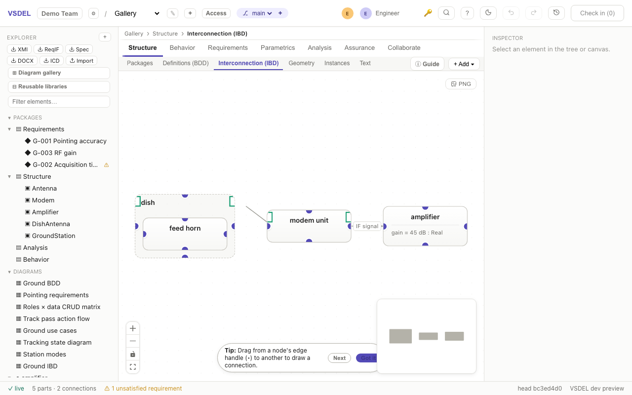
The Internal Block Diagram shows how part instances connect: parts (nested parts render inside their parents), ports on part boundaries, connectors between parts or ports, and item flows labelled with what moves. Drag part→part or port→port to connect; involve an item and the line becomes a labelled flow arrow. Drop a part onto another to nest it.
Use cases — who needs what
Frame the system: a system boundary rectangle names the subject; use cases (ellipses) go inside it; stick-figure actors stand outside. Drag actor↔use case to associate them (either direction works), use case→use case for «include», actor→actor for generalization. Drop a use case onto the boundary to move it inside.
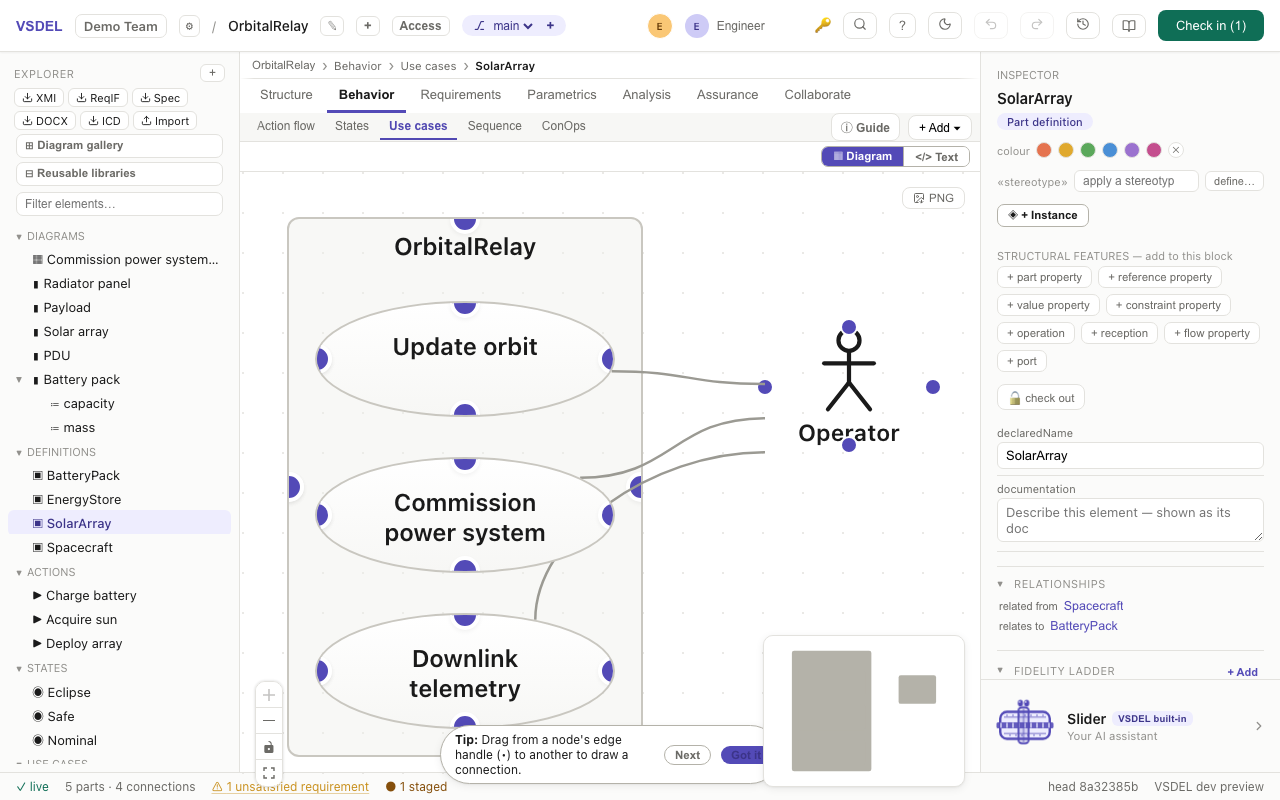
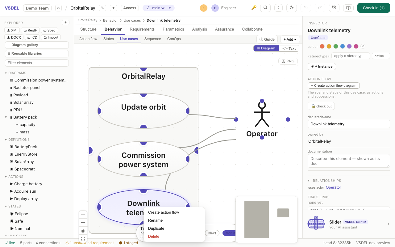
Decompose a use case into its scenario
In SysML v2 a use case is a kind of action, so its scenario is an action flow of its own steps. Right-click a use case (or use the inspector's ACTION FLOW section) → Create action flow; once it exists the same spots read Open action flow. Steps you add on that diagram are owned by the use case — a real decomposition.
Action flows — behavior as steps
Actions connected by successions (control flow), with decisions, forks, joins, and merges where paths split, and pins carrying object flow between actions. Guards on successions label conditional branches. Two terminators: the bullseye activity final ends the whole activity, while the circle-with-X flow final ends just one token. The ▶ Activity simulation panel token-walks the flow — and honors both, so a token reaching a flow final is consumed while parallel flows keep running.
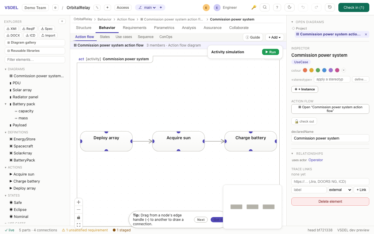
act [activity] … — its steps are owned by the use case or action it decomposes.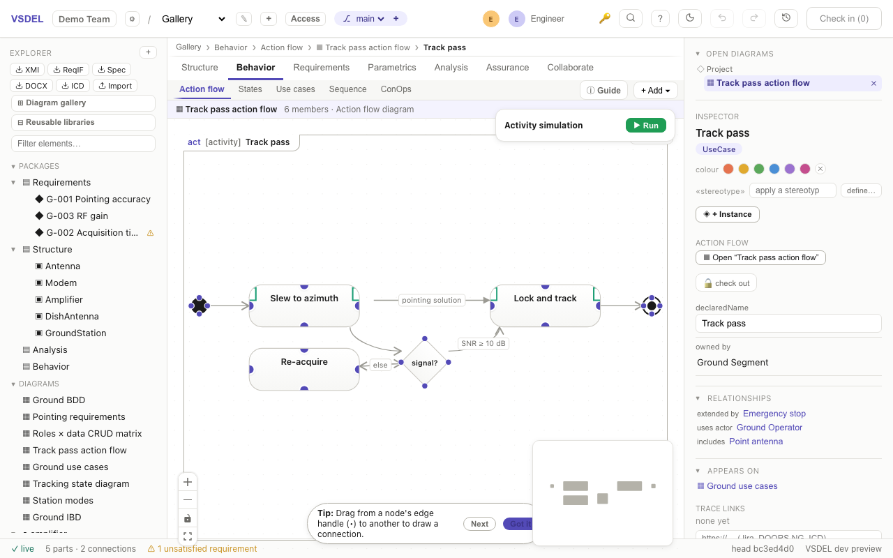
SNR ≥ 10 dB / else), and pins carrying an object flow.Recursive decomposition
Any action can decompose into its own lower-level flow: right-click → Decompose into action flow. Nodes that have a sub-flow show the ⋔ rake badge — the drill-down cue. One flow per subject, nested as deep as your model needs. Use SuccessionAsUsage for control edges here — TransitionUsage belongs to state machines and won't render on activity canvases.
States — modes and transitions
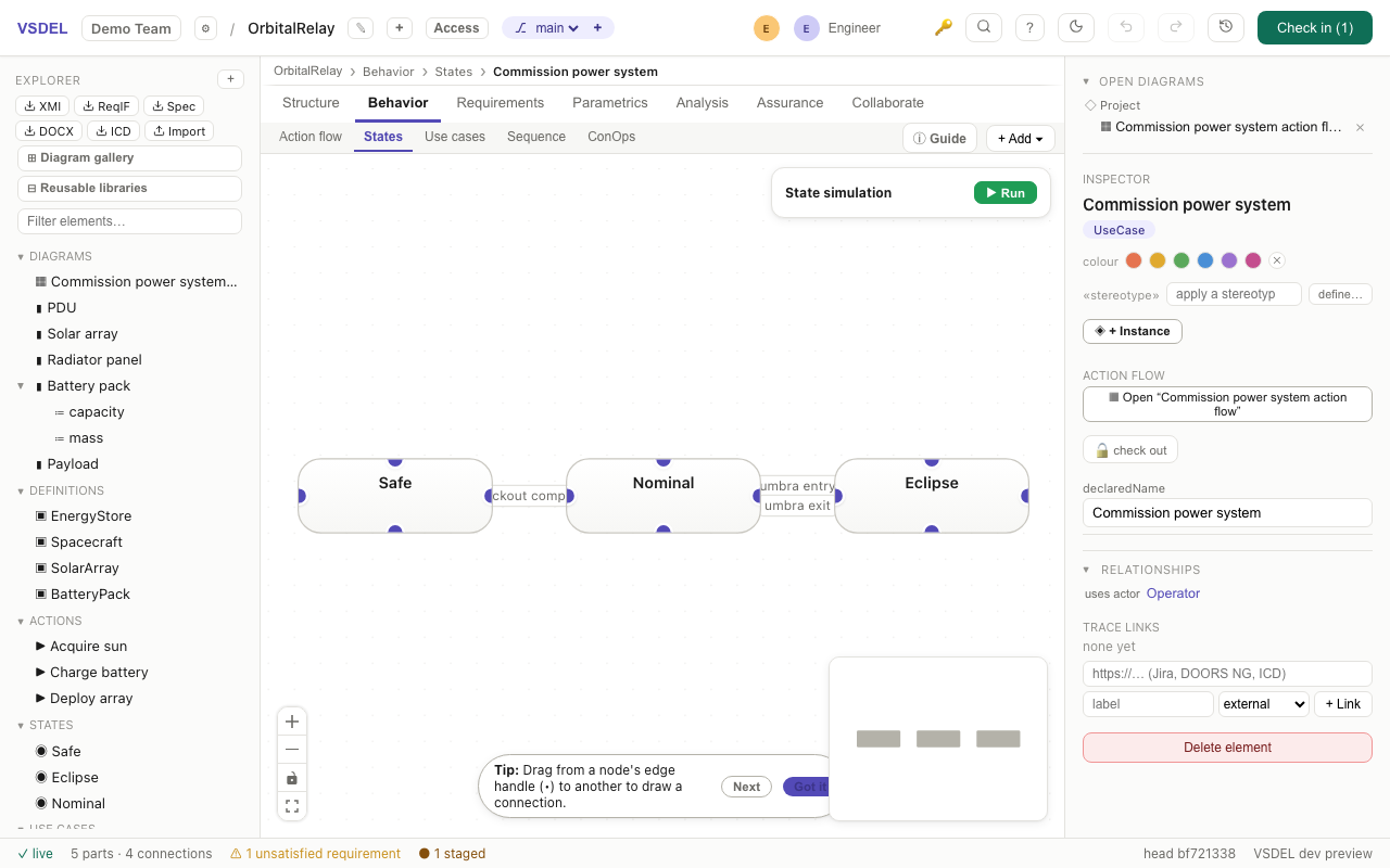
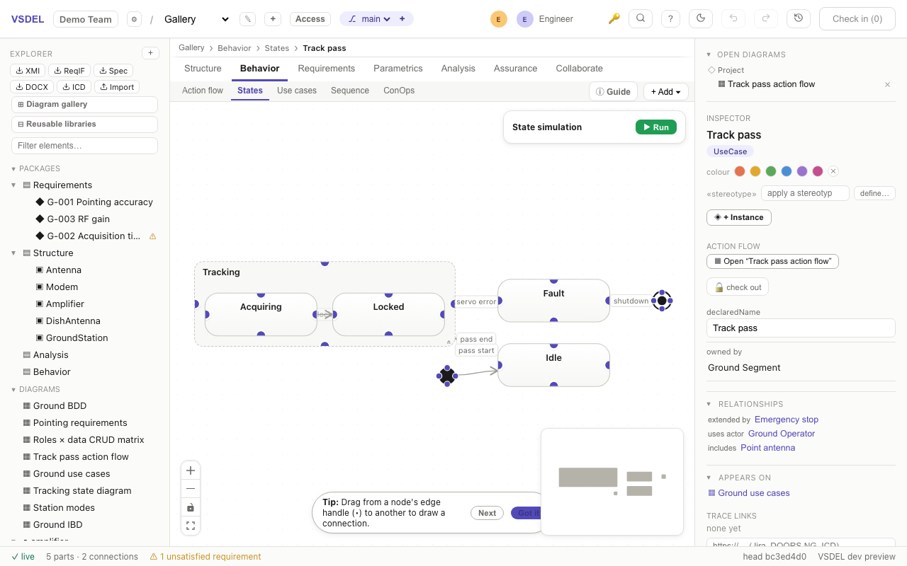
States (rounded), transitions with triggers, initial and final markers, and composite states. A composite state — one that owns substates — draws as a solid rounded region its substates nest inside. Nest substates directly, or right-click a state → Decompose into state diagram for a submachine of its own (⋔ badge on the parent). The state simulation walks transitions by trigger.
Instances — concrete configurations
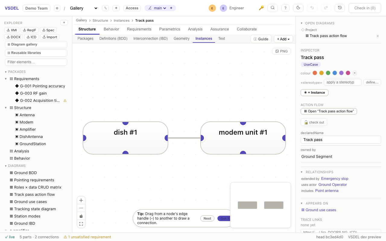
An instance specification is a specific configuration of a definition — this spacecraft, not the type. It draws in UML instance notation: its name and type render underlined (dish #1 : Antenna). Select a definition → inspector + Instance, fill slot values, link instances to each other. Slots are validated against the definition.
ConOps — the mission's operational phases
The ConOps (Concept of Operations) lens lays out a mission as a timeline of operational phases — launch, commissioning, nominal operations, safe mode, disposal, and whatever else the mission passes through — so the sequence and duration of what the system does is visible at a glance.
- Phases on a timeline: name each operational phase and place it in order across the mission.
- The operational narrative: capture how the system is intended to be used, from first activation through end of life.
- A shared reference: the phase breakdown gives every other lens a common vocabulary for when a behavior, mode or requirement applies.
When to use it. Use ConOps to frame the operational story early and keep it in view — it answers "what phases does this mission move through, and in what order." It is distinct from the Mission scenario lens: ConOps is the phase timeline, not the 3D orbital and coverage simulation. Reach for Mission scenario when you need the physics; reach for ConOps when you need the phased concept of operations.
Text — SysML v2 textual notation
Every graphical model carries a Diagram | Text toggle — flip any diagram to its SysML v2 textual notation in place (there is no separate Text tab to hunt for). It is not a separate document — it is the same model the graphical views show, so edits round-trip: type a change in the text and it appears on the diagrams; edit a diagram and the text updates to match. Packages render as nested package { … } blocks with their documentation.
- Read and author in text: express blocks, parts, requirements, states and the rest directly in the v2 language when that is faster than drawing.
- One model, two representations: the text is synchronized with the graphical views — no export step, no drift between the notation and the picture.
- Copy, paste & precise editing: select and reuse whole fragments of the model as text, and set exact names, types and multiplicities where a pointer is fiddly.
- Readable diffs: because the model has a textual form, a commit's changes read as a text diff in version history.
When to use it. Reach for the Text view when you are a power user who thinks in the language, when you want to bulk-author or paste structure faster than clicking, or when you are reviewing a commit and a line-by-line diff is clearer than a redrawn diagram.
Sequence — ordered interactions over time
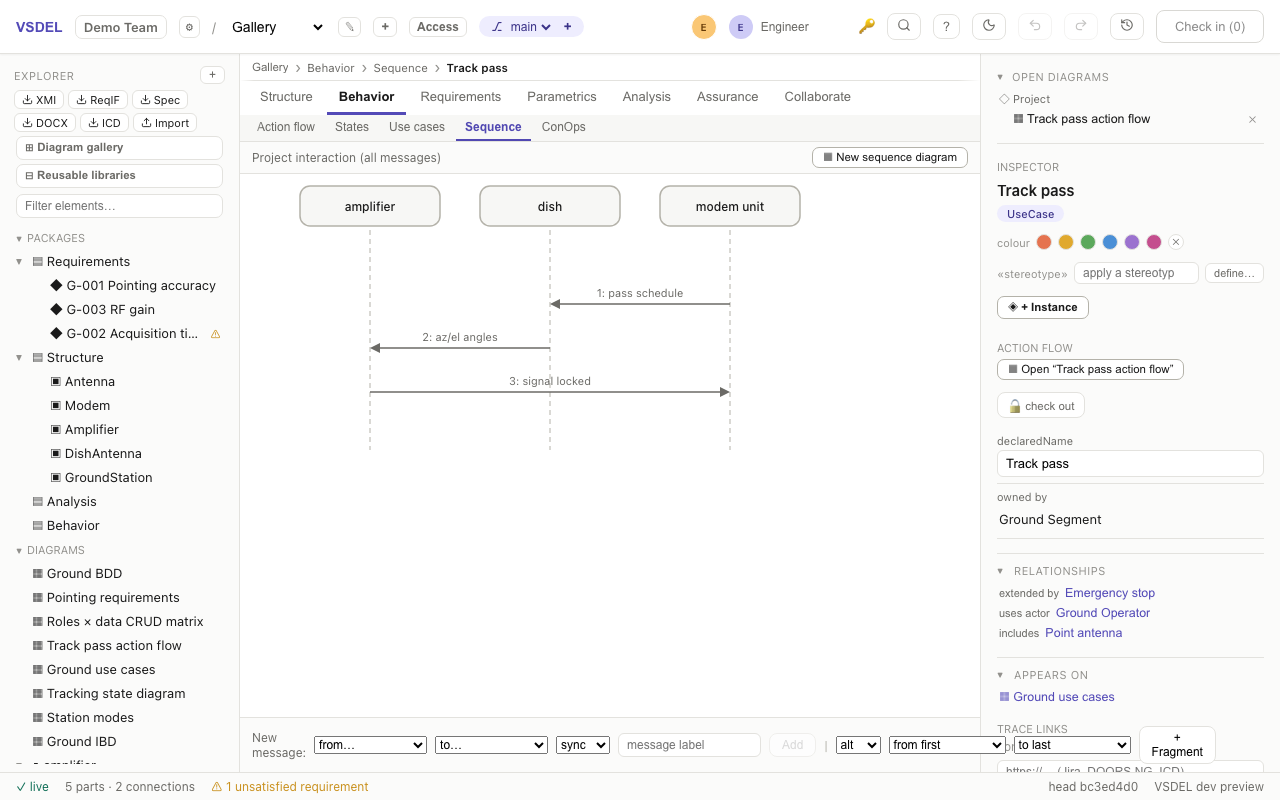
A sequence diagram (Behavior pillar) shows who talks to whom, in what order. Each participant is a lifeline drawn from a real part in your model, and messages run between them down the page — time flows top to bottom. Every named interaction is its own diagram, so one model can hold many scenarios (nominal startup, a fault response, a specific mission phase) side by side.
- Lifelines are your parts. Add a participant by picking an existing part, so the diagram stays connected to the model — rename or delete the part and the lifeline follows. Messages are ordered; reorder them to change the choreography.
- Messages carry intent. Name each message for the signal, command or call being exchanged, so the diagram reads as a protocol or a step-by-step exchange rather than a sketch.
- Combined fragments (alt / opt / loop) wrap a chosen run of messages in a labeled box. A fragment covers its messages, not row numbers — reorder the choreography and the box follows its content; if every covered message is deleted the fragment remains as a small chip you can select and remove.
- One interaction per diagram. Keep each scenario focused; the diagram list lets you jump between them.
When to use it. Reach for a sequence diagram when the order and direction of exchanges matters: a handshake or bus protocol between subsystems, the choreography behind a mode transition, an operational scenario walked step by step, or an interface's request/response timing. It pairs naturally with the Interconnection (IBD) view — the IBD says which parts are connected, the sequence says how they talk across those connections — and with Use cases, which name the goals a scenario satisfies. Where a single behavior is a flow of steps inside one part, an Action flow is the better fit; use a sequence when the story is the back-and-forth between parts.
Geometry — spatial layout & interference
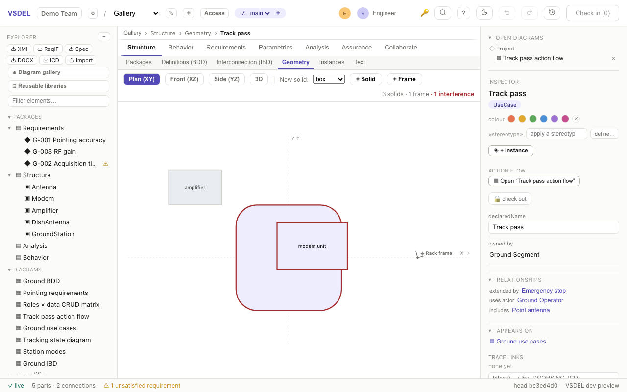
The Geometry lens (Structure pillar) gives your parts a shape and a pose (position and orientation) and lays them out in space — a lightweight packaging and layout study that lives on the same parts as every other view. See the arrangement as 2D plan / front / side projections or spin it in the WebGL 3D viewport, define coordinate frames to measure against, and let bounding-box interference checks flag parts that overlap.
- Shape & pose per part. Give a part a simple solid (box, cylinder, sphere…) and set its size, position and rotation. Because it is the same spatial part the CAD and Board lenses use, placement, mass and requirement budgets all carry through.
- Projections & 3D. Switch between orthographic plan/front/side for dimensioned layout work, or the 3D viewport to judge the arrangement as a whole.
- Coordinate frames. Define reference frames (vehicle, payload, sensor…) so positions and clearances are stated against a meaningful datum.
- Live interference. Overlapping courtyards are found by a bounding-box check and surfaced as findings in Model Health; the offending outline draws red so a fit problem is visible the moment it appears.
When to use it. Use Geometry early, for spatial reasoning before you commit to detailed CAD: rough packaging and envelope studies, checking reach and clearance, sanity-checking that everything fits inside the enclosure, or establishing the coordinate frames the rest of the model will reference. It is the low-fidelity rung of the spatial story — when you need real solids, booleans and STEP interchange, declare a CAD geometry realization on the same part (see the fidelity ladder) and move to the CAD lens; when the layout is a printed-circuit board, the Board lens is the specialized spatial view. Geometry keeps the whole thread connected from a first sketch to a released solid.
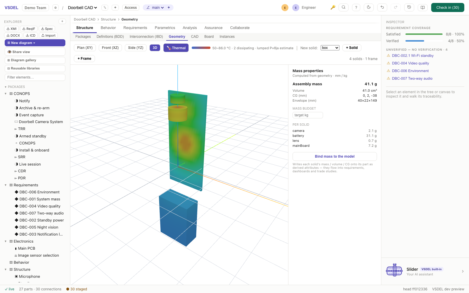
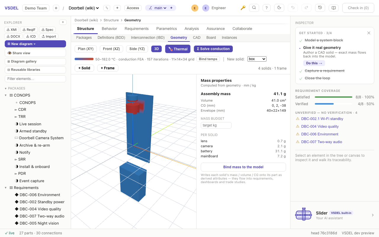
thermalConductivity, activePower and the declared ambient, with film convection at exposed faces. The legend reports the temperature range, iteration count and grid; Bind temps writes each part's computed max as a derived maxTempC attribute, so a requirement like max(maxTempC) <= 60 verifies against the solve.CAD — solid geometry (B-rep)
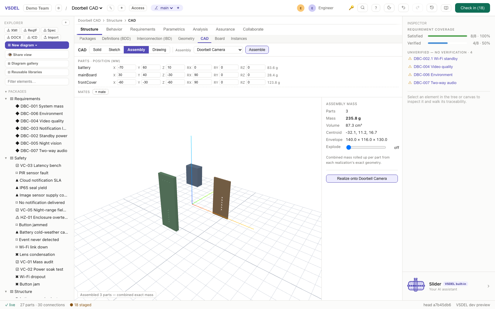
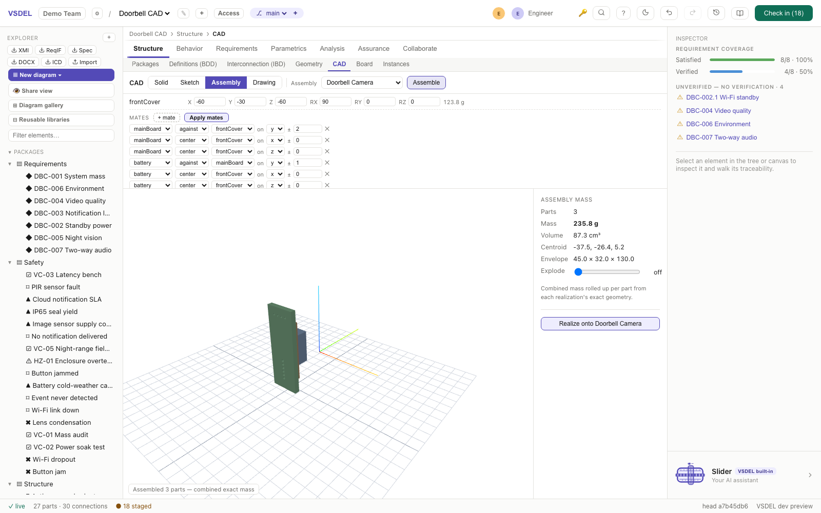
The CAD lens (Structure pillar) builds real B-rep solids on a full geometry kernel, so a part carries true watertight geometry rather than a bounding box. Author primitives (box, cylinder, cone, sphere), subtract positioned cut features — bores, recesses, connector notches, with linear patterns for hole rows and grilles and circular patterns for bolt circles — draw sketches on any datum plane (XY, XZ or YZ with an offset — side pockets and bosses without leaving the pad) — polygons whose edges bow into true circular arcs by dragging an edge handle, with dimensional constraints — extrude or revolve them, sweep them along a drawn path (tubes, ducts, bends), loft between sections (square-to-round transitions), or cut them straight into the existing solid (pockets and slots as ordinary patternable feature chips), drill standard fasteners with the hole wizard (ISO clearance, counterbore, countersink and tapped stacks that ring-pattern into bolt circles), dress up with fillets, chamfers and shells (all edges or picked edges), assign a material, and read the kernel's exact mass properties — volume, mass, centre of mass and envelope — in the same units the rest of the model uses. Assemblies position each realized child (with rotation), compute the combined exact mass, and open an instant exploded view; mate helpers (against / flush / center) place parts by intent instead of typed offsets — placements and mates persist as model elements, so the layout commits, branches and merges like everything else. Every assemble also runs an exact interference check (boolean intersection of the positioned B-reps); realizing the assembly binds the verdict onto the parent as derived attributes, surfacing clashes in Model health and making sum(interferenceCount) <= 0 a verifiable requirement. Dimensions accept expressions (=mass) bound to the model's attributes — geometry driven by the systems model — and the drawing sheet adds a hatched Section A–A with its cutting-plane trace, per-feature callouts, the kernel mass in the title block, and one-click exports as SVG, DXF (R12) and vector PDF — real deliverables for shop and review. Assembles also report near-miss clearances (the tightest pair gap binds as minClearanceMm), and Σ Solve conduction runs the ANA-7 thermal solve over the realized B-rep tessellations themselves — a shelled cover insulates like a shell — painting temperature contours on the assembly and binding each child's computed maxTempC. Σ Solve stress runs the same way: a quasi-static g-load elasticity solve (voxel finite elements, matrix-free) over the realized shapes with one face fixed — per-part peak von Mises and safety factor against the material yield, von-Mises contours in the viewer, and Bind SF staging minSafetyFactor so min(minSafetyFactor) >= 1.5 verifies structure the way mass, fit and temperature already verify. Σ Modes adds the first natural frequencies (lumped-mass subspace over the same voxel stiffness; firstModeHz binds — a disconnected assembly warns about its rigid modes instead of printing zeros), and Motion turns the mates' leftover degrees of freedom into travel studies: sweep a child through its range and the exact clash check runs at every pose, naming interference or binding interferenceFreeTravel. Materials carry E/ν/yield beside density and conductivity. Every material preset carries a real thermal conductivity beside its density, so picking "Aluminium" means aluminium physics everywhere — no silent defaults. Tolerance stack-ups live in the assembly panel: chains of contributor dimensions (each ± a tolerance, adding to or consuming the closing gap) persist as model elements, evaluate worst-case and RSS live with the largest contributor named, and Bind margin stages stackMarginMm so min(stackMarginMm) >= 0 verifies the fit like any other budget. The drawing sheet carries GD&T: feature-control frames (⌖ ⟂ ▱ + tolerance + datum) leadered to feature callouts, with the datum flag on the fixed face. Near-miss clearances report the true minimum surface distance (not a box approximation), part-to-part joints carry thermal contact resistance, and every feature chip suppresses (⏸ — the what-if lever: suppress a pocket, watch the budgets) and reorders.
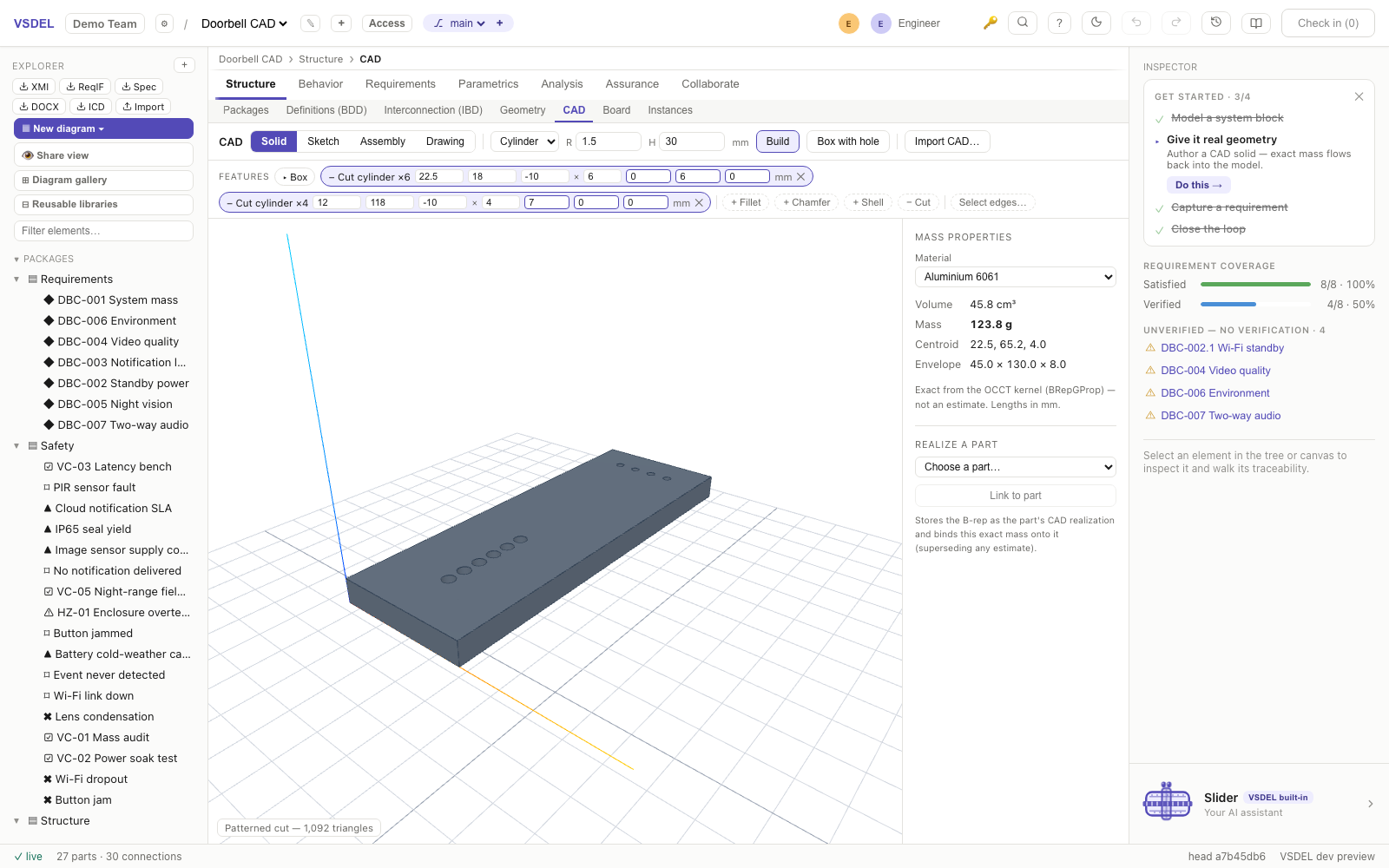
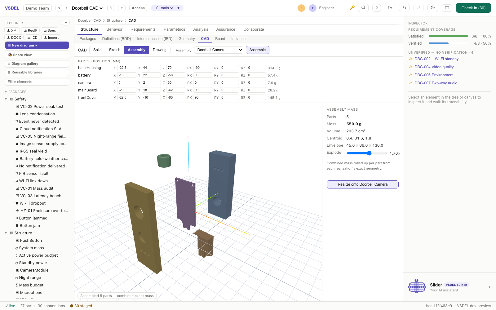
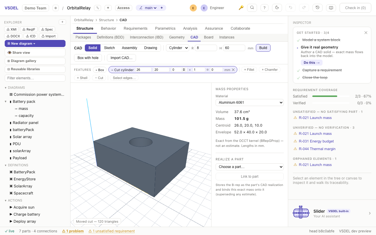
=mass into the width made this 52 × 40 × 20 plate — the value came from the model's own attribute, and when the model changes, the solid regenerates. A positioned cylinder cut bores the centre; the kernel's exact volume and mass update live.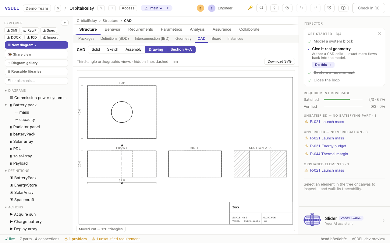
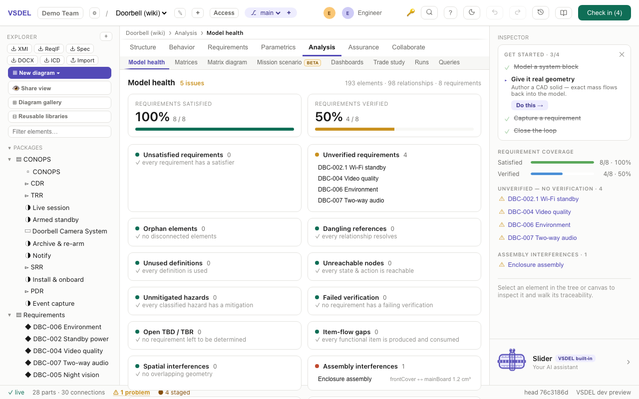
interferenceCount / interferenceVolume onto the parent, and Model health reports the pair — here frontCover ↔ mainBoard, 1.2 cm³ — one click from the offending part. A clean realize binds zeros, which is itself the verifiable no-interference fact.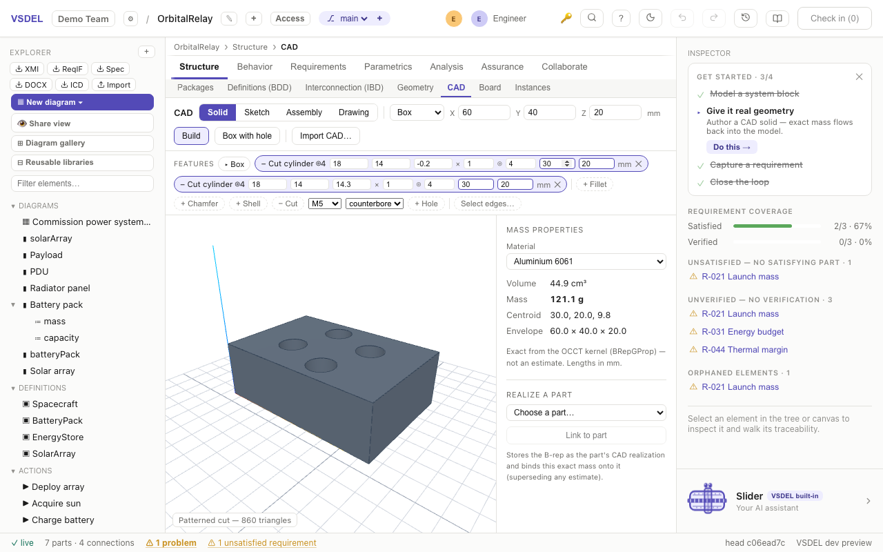
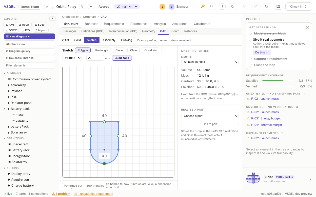
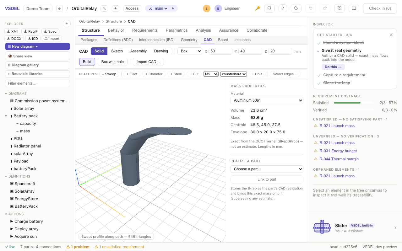
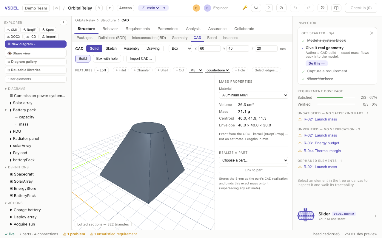
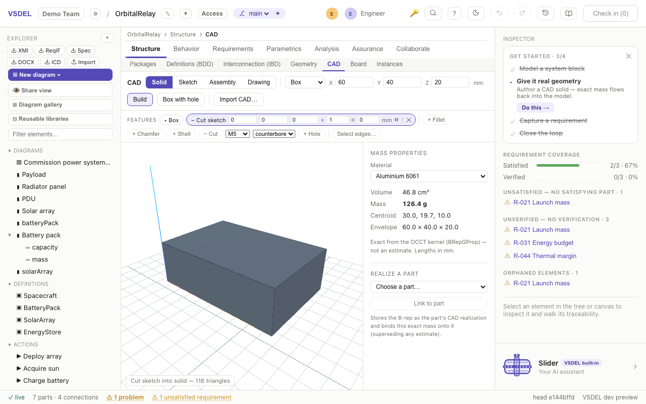
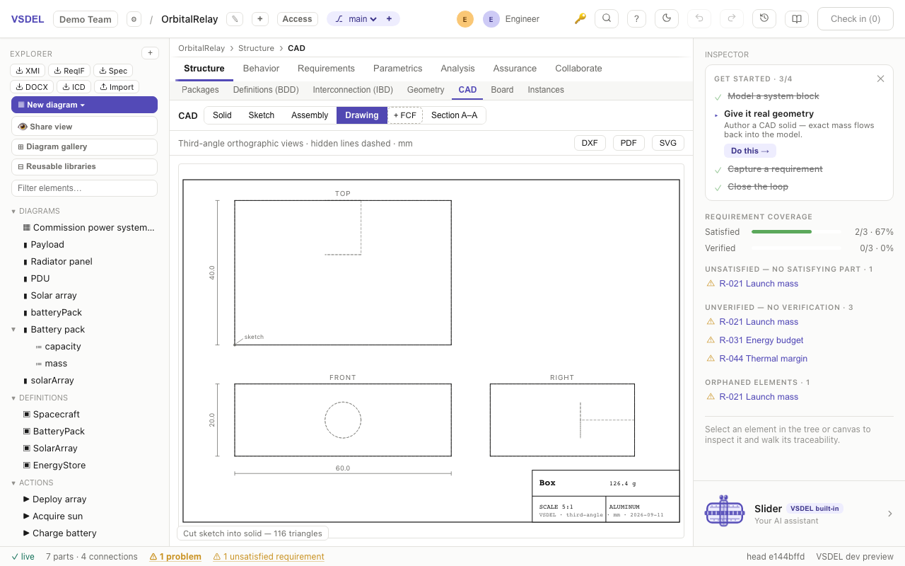
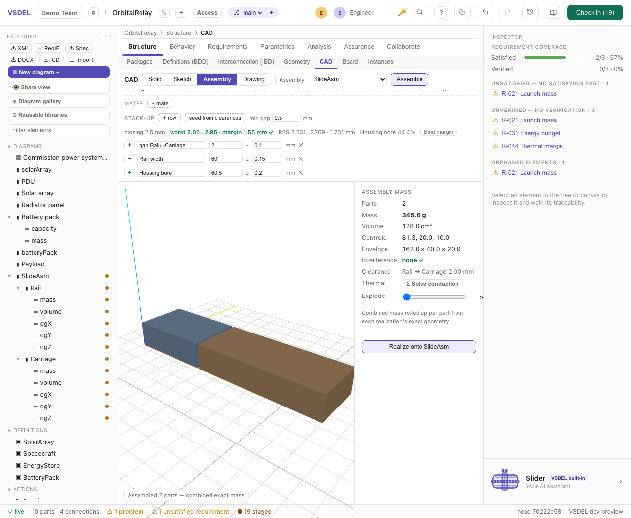
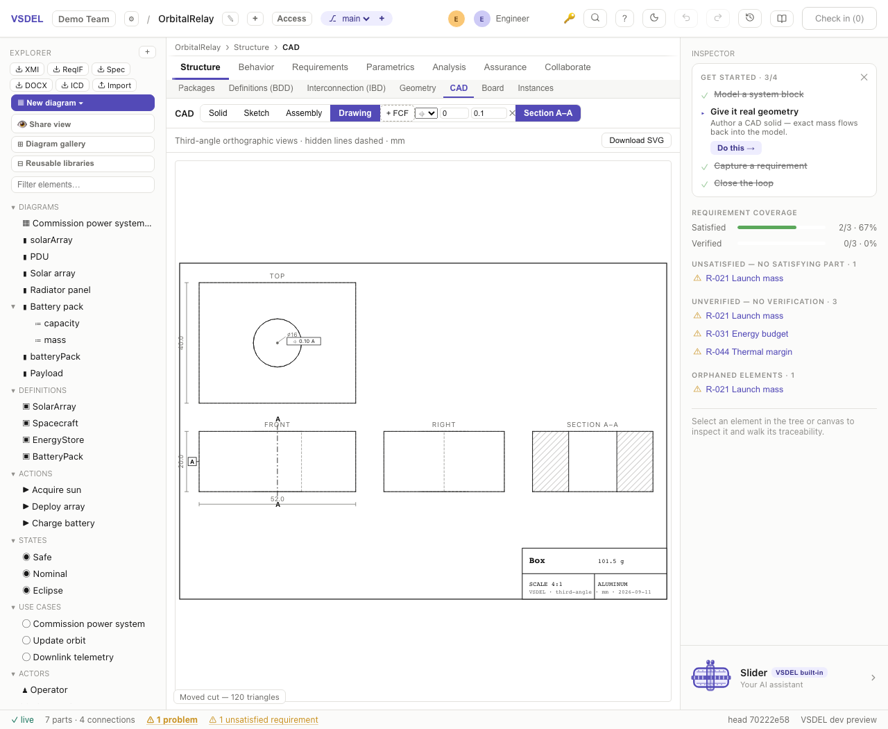
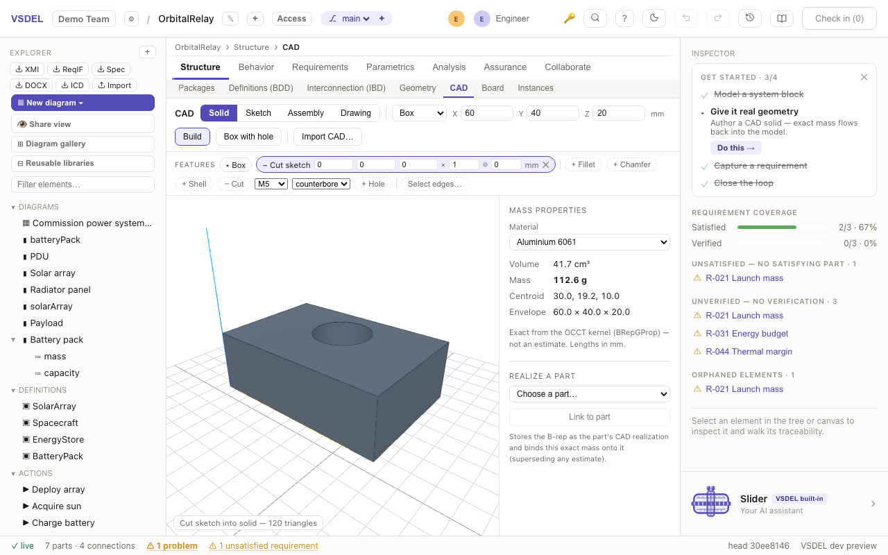
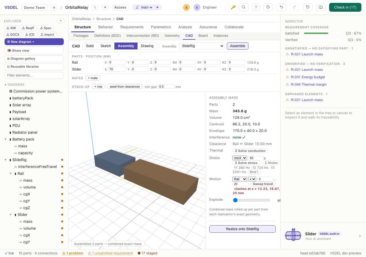
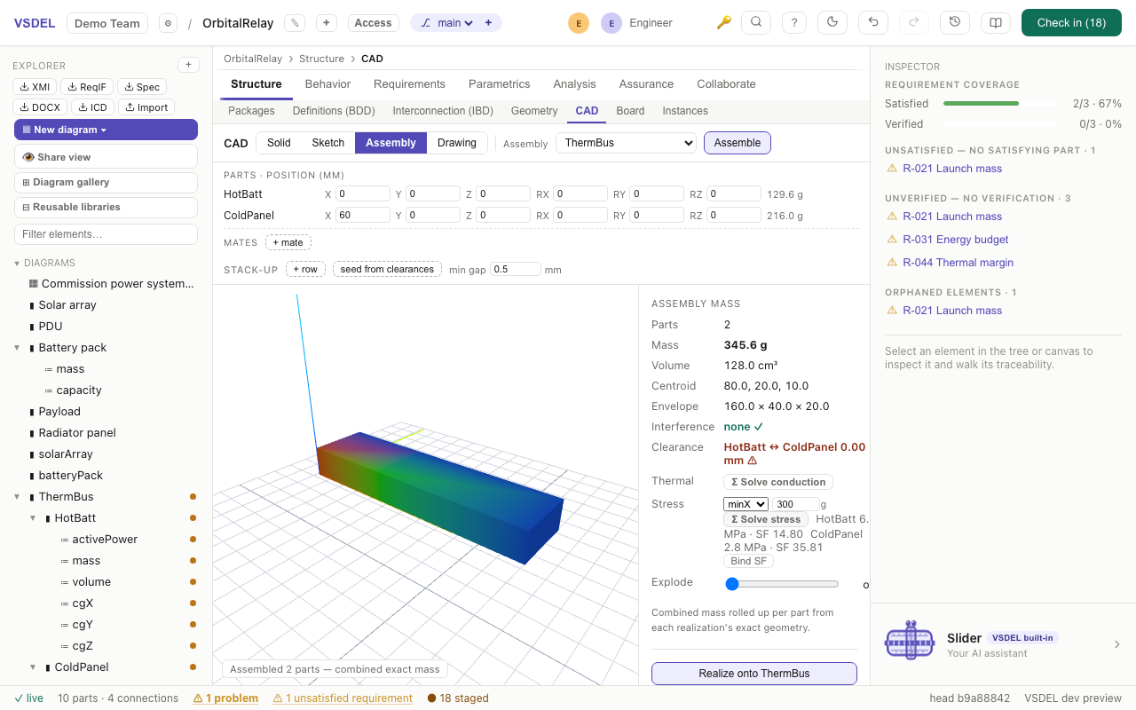
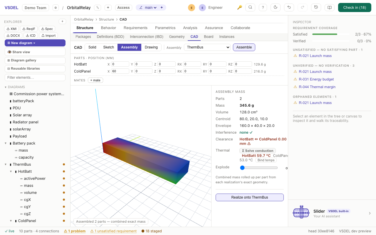
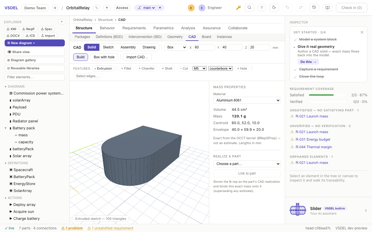
- Primitives, booleans & sketches: place parametric primitives, cut or fuse them into the real shape, and build features from 2D sketches — the kernel evaluates the true solid, not an approximation.
- Import STEP / IGES / BREP: bring a supplier or mechanical-CAD model into the systems model, tessellated for display, with its mass properties read straight from the solid.
- Materials & exact mass: pick a material and density; volume, mass, centroid and envelope come from the B-rep and roll up into the model's mass budgets.
- Assemblies & drawings: combine parts into a compound with a per-material mass roll-up, and generate a dimensioned drawing sheet from the solid.
- Same spatial part: a CAD solid lives on the same part the Geometry, Board and mass views share, so pose, placement and interference stay consistent across lenses.
When to use it. Move to the CAD lens when a bounding box is no longer enough — you need the real shape for fit, mass, clearance, or to exchange geometry with mechanical CAD. It is the higher-fidelity rung above the Geometry lens (quick spatial layout): start rough in Geometry, then declare a CAD geometry realization (see the fidelity ladder) and author or import the solid here. For a printed-circuit board, use the Board lens instead — the specialized spatial view for PCBs.
Limitations. This is solid modeling for the systems model — primitives, positioned cuts with patterns, sketches, per-edge dress-ups, drawing sheets and STEP/IGES/BREP import, with exact mass — not a replacement for a full production mechanical-CAD suite: expect a lighter feature history than a parametric MCAD tree, and assembly mate helpers (a placement calculator) rather than a full constraint network. No surfacing, sheet metal or CAM. For detailed mechanical design, author in a dedicated MCAD tool and exchange via STEP.
Board — PCB planning
The Board lens (Structure pillar) plans a printed-circuit layout on the same model your other views share. Choose a board part, and its child parts become components you place on the outline; connections between them draw as a live ratsnest. It is a planning environment, not a router — the copper is left to KiCad.
When to use it. Reach for the Board lens to plan a PCB inside the systems model — while the electrical architecture is still connected to requirements, mass and cost — rather than as a standalone ECAD project. It is the right home for early placement and floor-planning (does the part set fit the outline? where do the connectors go?), for turning model connections into a netlist, for sanity-checking spacing, net classes and a rough layer/via count before routing, and for producing a costed, manufacturable BOM. When the plan is ready you hand it to KiCad for the actual copper — so think of this as the placement-and-connectivity stage of PCB design, kept in the same repository as the rest of your system.
- Import / export KiCad: bring in a
.kicad_pcbboard or.netnetlist — outline, footprints, placement and nets — then export back to.kicad_pcb/.netpin-accurately for routing, plus a BOM as CSV. - Real footprints & pads: a curated footprint library (chip, SOIC/TSSOP, QFN/TQFP, headers…) gives each component real pads; nets connect pad-to-pad, and a Pads→nets list shows each pad's net.
- Design-rule checks: edge clearance, courtyard spacing, keep-out zones, pad-to-pad shorts and dangling nets — offenders highlight red, live as you drag.
- Net classes & routing: assign trace width and clearance per class (power rails auto-classified), pick each net's topology (minimum tree, star or daisy-chain), length-match differential pairs and buses against a tolerance, and set a route-to-length target that shows the meander each net needs. A layer & via estimate reads the routing congestion for a quick stackup sanity check.
- Costed BOM & CSV export: components group by value + footprint + part number into a bill of materials with unit and extended cost, a per-board and build-quantity total, and a one-click CSV. The CSV is a full manufacturing + purchasing document — each line carries References, Qty, DNP, Value, Description, Footprint, Side, Manufacturer, MPN, Alt MPN, Lifecycle, RoHS, Rating, Height, MSL, ECCN, Datasheet and Notes, plus Supplier, Supplier Part No, Stock, Stock Updated, MOQ and Lead time once you add sourcing. Most of these come straight from the imported KiCad properties/fields; the rest are editable per component in the inspector.
- DNP (do-not-populate) parts are captured from the footprint's
dnpattribute (or a checkbox), listed with a DNP marker, and excluded from the ordered quantity and cost — placement, not purchase. - Sourcing: type supplier / stock / MOQ / lead time per line, or import a supplier CSV (Digi-Key/Mouser/ERP export) matched by part number — it also pulls unit price, distributor SKU, RoHS and lifecycle, and stamps a stock date. The build is flagged where stock falls short of what it needs.
- DNP (do-not-populate) parts are captured from the footprint's
Import & export. The Board lens round-trips pin-accurately. Import a .kicad_pcb (board outline from Edge.Cuts, footprints with placement and real pad geometry, pad nets, footprint names matched to the library, component values and net_class blocks) or a .net netlist (components and node pins, auto-placed) — KiCad's Y-down coordinates are flipped to the board's Y-up. Export back to a .kicad_pcb with the outline, every component's real footprint pads bound to their exact net at the pad level, net-class blocks and values, plus a .net netlist for "Update PCB from netlist" — so you route in KiCad and can bring changes back. The costed .csv BOM is the third export. Round-trips are covered by tests that export, re-parse, and confirm the board, placement, named nets, footprints and classes all survive.
Limitations. This is placement and connectivity planning, not copper. There is no track routing or autorouting, no copper design-rule check (clearance / annular ring / manufacturing rules), no layer stack-up editor, and no Gerber or drill output — those belong to a dedicated ECAD tool. Net "length" is the straight-line ratsnest length (a planning proxy for trace length), not a routed length, and the layer/via figure is a heuristic estimate from routing congestion, not a routed result. The footprint library is a curated set (chip, SOIC/TSSOP, QFN/TQFP, SOT, headers…); a part outside it imports under its raw footprint name. In short: plan, validate, cost and hand off — do the routing and fabrication output downstream.
Requirements
Requirements live in two synchronized places: the requirements table (unique IDs, rich text, custom attribute columns, rationale, saved views, package-scoped levels, e-signature approvals) and the requirement diagram (boxes with «satisfy»/«derive» traces). Every requirement shows a live ⚠ until something satisfies it.
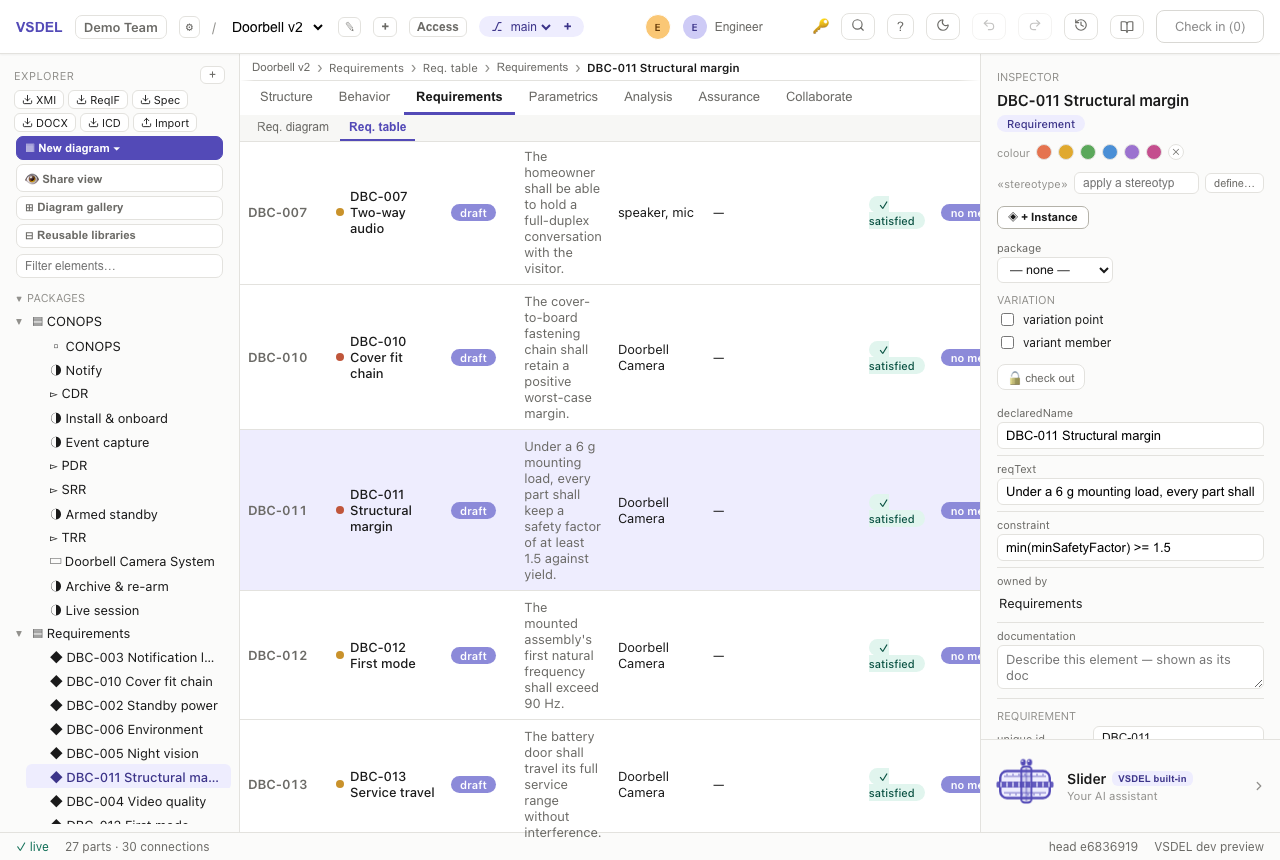
min(minSafetyFactor) >= 1.5, evaluating 14.8), the first mode (380 Hz ≥ 90), and interference-free service travel. Re-run any solve and the verdicts refresh.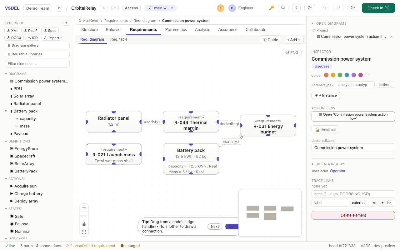
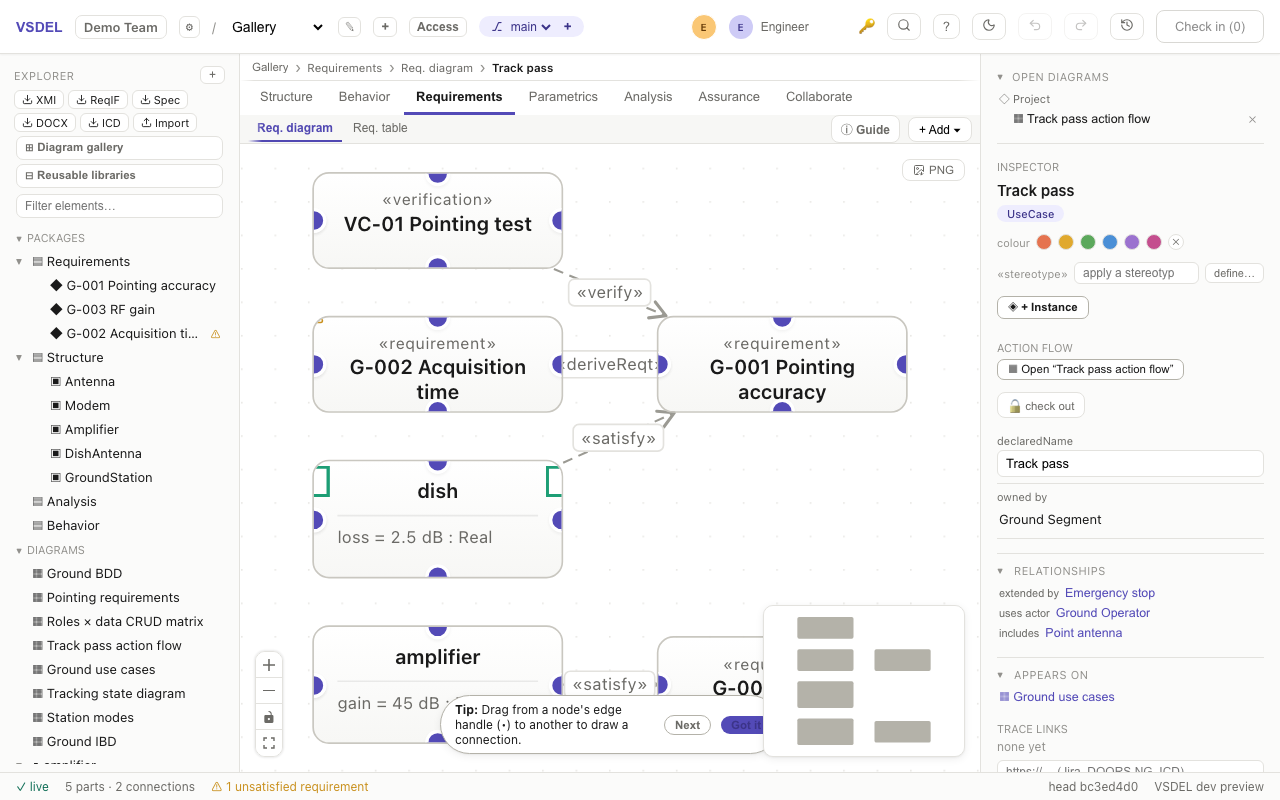
- Notation: each «requirement» box shows its short-name
idand a labelledtextcompartment, the way SysML v2 draws it. - Satisfy: drag a design element → requirement (diagram) or use the trace tree.
- Verify: "+ V&V" on a table row stages a verification case wired to the requirement.
- Suspect links: editing a requirement's text flags its traces ⚠ until re-confirmed.
- Derivation: requirement → requirement «derive»; switch stereotype (refine/trace/copy…) in the inspector.
- Export & upload: the table's ⬇ CSV / ⬇ Excel buttons export the current (filtered) view; ⬆ Import uploads a CSV/Excel back — rows matched by ID, edits and new requirements staged for review.
Parametrics & computed verification
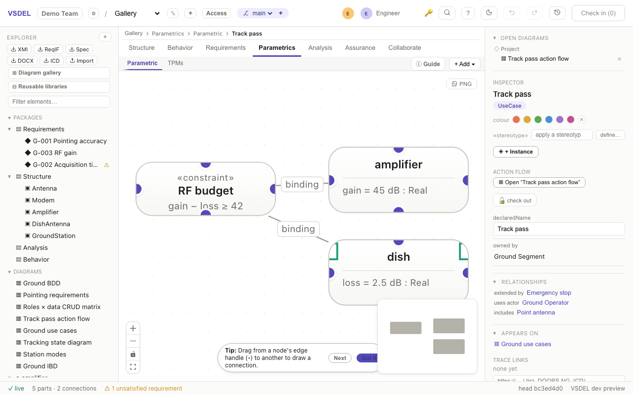
Constraint blocks hold equations; a constraint's parameters render as small boxes on its boundary, and a binding connector pins a part onto a specific parameter. The unit-aware solver then computes verification verdicts: a mass budget reads ✓ 2.48 kg ≤ 2.5 and recomputes on every commit. Give values units in the inspector.
Bindings feed the result. Drawing a binding is not just a trace — it scopes the evaluation: a constraint bound to specific parts computes over just those parts, so the same expression can read a subsystem's budget rather than the whole model's. An unbound constraint falls back to the whole-model roll-up (aggregated over composition).
TPMs — technical performance measures
Technical Performance Measures track the key engineering parameters that decide whether the design is on course — mass, power, latency, and the like — each as a current value against a threshold (the value that must be met) and an objective (the value aimed for), with the margin computed for you.
- Current vs. threshold vs. objective: state where a parameter stands today against both the must-meet and the target values.
- Computed margin: see how much headroom remains before a measure breaches its threshold.
- Trends with the model: as the design changes, a TPM's current value moves, so a tightening margin shows up as it happens.
When to use it. Track a TPM for any parameter whose margin you need to watch across the program. TPMs pair naturally with Parametrics & computed verification — a solved roll-up such as a live mass budget is exactly the kind of computed value that feeds a measure — and with the requirements that set the threshold in the first place.
Matrix diagrams — rows × columns × relationships
The classic dependency/allocation matrix as a named diagram (Analysis → Matrix diagram): pick a row set and column set — elements specializing a root (a role tree), children of a category block, or an explicit list — and cells show the relationships from the row element to the column element (association endLabel text, e.g. CRUD grants). Rows inherit their ancestors' cells down the specialization tree (shown muted, with the source on hover), scrolling keeps the headers frozen — which is what makes a role hierarchy readable as one table instead of six diagrams.
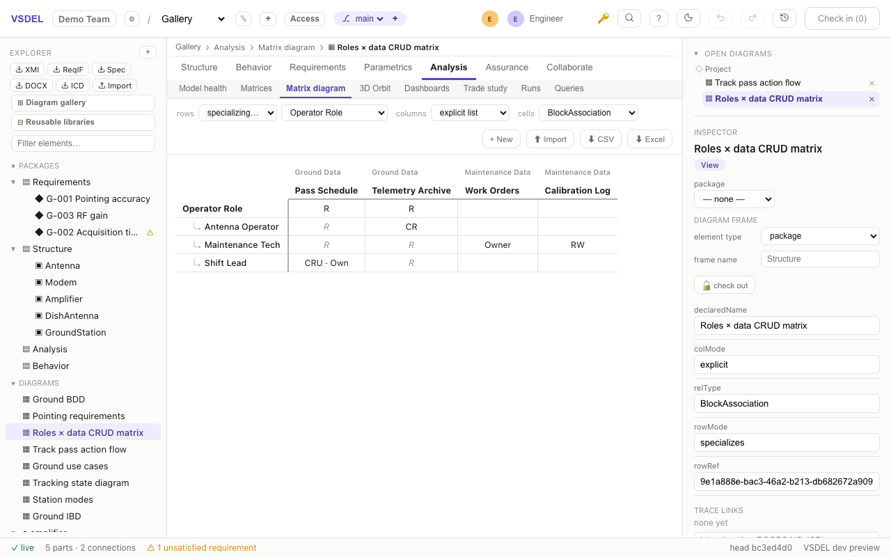
- The role tree is visible: parents render bold, children carry a ↳ with depth indentation and a hover tooltip naming what they specialize — and this works whatever way the rows were picked (explicit lists included), because the hierarchy is read from the model's specialization relationships, not the axis mode.
- Keep as many matrices as you need: each is a named diagram persisting its own rows, columns, and relationship type — the toolbar's + New creates another, and all of them live in the explorer, gallery, and version history like any diagram.
- Edit in place: double-click any cell to write its label — updating the relationship, or creating it if the cell was empty. Everything stages for review like any edit.
- Crosshair: clicking a cell lights up its row and column headers (and faintly tints both lanes), so you always know exactly which row × column intersection you're editing, however wide the matrix.
- Export: ⬇ CSV or ⬇ Excel (a real .xlsx) of the live grid, inherited cells marked with *.
- Upload: ⬆ Import a CSV/Excel table back — rows and columns matched by name, differences staged (new relationships created, labels updated); unchanged and inherited cells are left alone.
Mission scenario analysis
The Analysis pillar's Mission scenario lens is a multi-domain mission simulation. The model carries the design — and every element declares how it moves through typed attributes: satellites on orbits, aircraft/ships/vehicles on waypoint routes, fixed sites. One scenario mixes them all. Scenarios are persisted artifacts, like trade studies: each picks participants, overrides parameters, sets start time and span, and chooses the propagator — exercising the model without changing it.
| Attributes on a part (the design) | Becomes |
|---|---|
altitudeKm (or semiMajorAxisKm), + optional inclinationDeg, raanDeg, eccentricity, argPerigeeDeg, trueAnomalyDeg | An orbiting platform |
routeWaypoints ("lat,lon; lat,lon; …") + speedKmh, + optional routeAltitudeKm, routeLoop | A route mover (aircraft, ship, vehicle) flying great-circle legs |
latitudeDeg + longitudeDeg, + optional minElevationDeg (default 5°) | A fixed site with an elevation mask |
sensorConeDeg, + optional sensorRangeKm | A nadir-pointing sensor — detects sites and other movers |
centralBody ("moon", "mars", "sun") + orbital attributes | An orbit around another body — e.g. a lunar relay at 100 km |
transferTo ("moon"…), + transferDepartHr, transferDurationHr, transferArrival ("land" / "orbit"), arrivalAltitudeKm | A transfer mission: parking orbit, guided cruise, then landing (near side) or orbit capture |
- Photoreal model store: an instance admin can upload a photorealistic model (binary glTF
.glb) per element kind in the Admin panel's 3D models tab. Uploaded models are served from the instance's own origin — no CDN — so the strict client CSP and the air-gapped self-host edition keep working; kinds without an upload use the built-in procedural model. - 3D models: every element renders as a recognizable 3D model on the globe — satellites with solar wings and dishes, aircraft and fighters with swept wings, helicopters with rotor disks, ships and submarines with hulls and sails, ground vehicles, and ground-station dishes — oriented along the velocity vector so movers point where they travel. (Models are built procedurally so the whole tool stays offline and self-contained.)
- Three views, one continuous scene — transitions are smooth camera flights, never hard cuts: Space frames the Earth, the Earth–Moon system, or the whole System when a mission goes celestial; Sky flies the camera above any observer looking straight down, so aircraft and ground assets read like a live map; Element eases into tracking one element with its live position, altitude and speed.
- Beyond Earth: missions extend to the Moon, Mars and heliocentric space — orbits around other bodies, and transfer missions (launch from a parking orbit, a guided cruise that chases the moving target, then a near-side landing or orbit capture). The Moon and Mars occlude line of sight, and the deep-space geometry follows the scenario's start date. Ephemerides are visualization-grade circular mean orbits — right scale and period.
- Template elements: pull ready-made platforms into the model from the lens — imaging (SSO), GEO comms and LEO broadband satellites, ISR aircraft, fighter jet, helicopter, long-endurance drone, ship, submarine, ground vehicle, ground station. Each stages a real model subtree: the platform part with movement attributes plus subsystem parts carrying their own typed attributes. A separate Add payload picker attaches more sub-elements to whichever element is selected — EO/IR sensors, SAR, surveillance radar, SIGINT, Ka/UHF/optical comms, SATCOM, tracking antenna, GNSS — all reviewed and checked in like any edit, and equipping the platform in the analysis. Weapon sub-elements (air-to-air / air-to-ground / cruise / anti-ship missiles, guided bombs, SAM, torpedoes, naval gun, CIWS) attach the same way, as modeled loadout parts with range and quantity attributes.
- Tailor and save for reuse: every attribute on a platform or sub-element is a real, editable model value — change altitude, sensor cone, weapon range, data rate, anything. Then Save as template captures that element with its whole subsystem subtree and tailored attributes as your own reusable template, which appears in Add element under "Saved" for stamping into any scenario or project.
- Scenario time: each scenario has a start date-time and span (6 hours to 7 days); watch in real time (1×) or accelerated (60× / 600× / 1800×), pause, and scrub anywhere in the span. Click a pass in the access table to jump the clock to it.
- Scenarios like trade studies: create as many as you need (+ New); participants, situation overrides ("what if 700 km?"), start, span and propagator persist on the scenario artifact — versioned and reviewed like everything else. Save results stores windows and per-pair metrics on it for side-by-side comparison.
- Physics by default: orbital elements integrate the two-body + J2/J4 zonal field numerically (sun-synchronous precession ≈0.99°/day is emergent); two-body Keplerian is selectable; Load… accepts a user-defined propagator (
propagate(orbit, tSeconds) → [xKm, yKm, zKm]) that runs only in your browser session. Access analysis covers site↔mover passes, mover↔mover crosslinks with Earth occlusion, and sensor detections — including events shorter than a sampling step. - Start fast: the Constellation mission sample mixes three relays, a patrol aircraft, two ground stations and sensors; the Lunar transfer mission sample launches a crew vehicle from Earth parking orbit to a Moon landing with a lunar relay orbiter and the three-site deep-space network.
Parts without movement attributes still fly as a default LEO train so any structural model gets a live globe.
Analysis & assurance lenses
The Analysis and Assurance pillars read the same model: Model health (coverage gauges, orphans, dangling references — every finding one click from its element), matrices (dependency + editable allocation; for a configurable, exportable rows × columns table see Matrix diagrams), dashboards, queries, FHA (severity→DAL), FMECA (S×O×D→RPN), fault trees, a 5×5 risk register, TPMs, lifecycle review gates, trade studies, and a ConOps mission timeline.
Dashboards — Visualization Studio
The Dashboards lens is a Visualization Studio for building trade-study dashboards with charts (powered by ECharts) over your model and trade-study data — a place to see the numbers and compare alternatives visually rather than reading them off a table.
- Charts over model data: visualize values drawn from the model and from study results.
- Trade-study dashboards: assemble charts into a dashboard for comparing options side by side.
- ECharts rendering: a full charting library backs the plots.
When to use it. Build a dashboard when you want to see a comparison — weighing alternatives from a trade study, plotting the time-series a co-simulation run produced, or presenting how a set of measures stands. It is the visualization surface for the analysis lenses.
Trade study — weighted decision matrix
The Trade study lens is a weighted decision matrix: define the alternatives you are choosing between and the criteria that matter, weight the criteria by importance, score each alternative against each, and read a ranked recommendation.
- Alternatives × criteria: lay out the options against the factors that decide between them.
- Weighted scoring: assign each criterion a weight and score every alternative, so the ranking reflects what matters most.
- Ranked result: the matrix rolls the weighted scores into an ordered recommendation.
- Persisted as an artifact: the study is saved with the model, so the decision and its rationale live alongside everything else.
When to use it. Reach for a trade study whenever a design decision comes down to a defensible choice among options against weighted criteria — architecture selection, component choice, a build-vs-buy call. Feed it hard numbers from a co-simulation run, and visualize the comparison in a dashboard.
Runs — FMU co-simulation
The Runs lens executes FMU co-simulation runs and shows the resulting time-series. An FMU (Functional Mock-up Unit, from the open FMI standard) packages a simulation model; running one exercises the behavior over time and produces data the rest of the analysis lenses can use.
- Execute FMU runs: drive a co-simulation from the model and collect its output.
- Time-series results: view how the simulated quantities evolve over the run.
- Feeds studies & dashboards: run results become inputs to trade studies and are plotted in dashboards.
- Open-standard interop: FMI/FMU is an open co-simulation interface, so models from many sources can be run here.
When to use it. Use Runs when a decision needs simulated behavior rather than a static number — dynamic response, transient performance, anything an FMU computes over time. The time-series it produces is the quantitative backbone for a trade study or a dashboard.
Queries — saved model queries
The Queries lens holds saved, re-runnable queries over the model, expressed through the OMG Systems Modeling API (the standard programmatic interface to a SysML v2 model). A query finds the elements matching a set of constraints; saving it means you can run it again, and share it, without rebuilding the search.
- Find by constraint: return the elements that match the conditions you specify.
- Save and re-run: keep a query as a named artifact and execute it again whenever you need the current answer.
- Reuse and share: a saved query is available to the team, so a useful search is written once.
- Standard API: queries run over the OMG Systems Modeling API, the same standard interface used for programmatic access.
When to use it. Save a query for any question you ask of the model more than once — "every requirement without a satisfy," "all parts over a mass threshold," "elements owned by this package." It turns an ad-hoc search into a reusable, shareable check.
Safety — Functional Hazard Assessment
The Safety lens runs a Functional Hazard Assessment (FHA): identify the system's functions and the hazards associated with their failure, assign a severity to each, and derive the Development Assurance Level (DAL) the function must be developed to — following ARP4754A.
- Functions & hazards: enumerate the functions and the hazardous conditions that a failure could cause.
- Severity classification: rate the consequence of each hazard.
- DAL derivation: turn severity into the assurance level required, per ARP4754A.
When to use it. Use the Safety lens on safety-relevant systems to establish, early and traceably, how rigorously each function must be developed. The DALs it produces set the assurance targets that flow down into the rest of the program's safety work.
FMECA — failure modes & effects
The FMECA lens supports FMEA / FMECA: enumerate the ways parts and functions can fail, rate each failure mode for Severity, Occurrence and Detection, and compute the Risk Priority Number (RPN = S × O × D) so the worst modes rise to the top.
- Enumerate failure modes: capture how each element can fail and what the effect is.
- Rate S × O × D: score how bad, how likely, and how detectable each mode is.
- Compute RPN: multiply the ratings into a single priority number.
- Prioritize: rank the failure modes by RPN to focus mitigation where it counts.
When to use it. Run an FMECA to systematically work through a design's failure modes and decide which ones warrant action first. It complements top-down analyses like the fault tree: FMECA reasons bottom-up from individual failures, the fault tree reasons down from a top-level event.
Fault tree — top-down failure logic
The Fault tree lens builds a Fault Tree Analysis: start from a top event (the failure you care about) and decompose it downward through AND / OR gates to the basic events that can cause it, then roll up probability from the basic events to the top.
- Top event down to basic events: model the logical chain from a system-level failure to its root causes.
- AND / OR gates: express whether causes must combine or any one suffices.
- Probability roll-up: assign probabilities to basic events and propagate them up the tree to the top event.
When to use it. Reach for a fault tree when you need to reason from a specific undesired outcome back to its causes and quantify how likely it is. It is the top-down counterpart to the bottom-up FMECA, and pairs with the Safety lens's hazard work.
Risk — register & 5×5 matrix
The Risk lens is a risk register that scores each risk on a 5×5 matrix of likelihood × consequence, giving a rated position from low to high, and tracks the mitigation for each.
- Register of risks: keep every identified risk in one place.
- Likelihood × consequence: score each risk on the 5×5 grid for a consistent, comparable rating.
- Mitigation tracking: record the action being taken against each risk and follow its status.
When to use it. Use the Risk register as the program's standing view of what could go wrong and what is being done about it — technical, schedule or programmatic risks alike. Where the Safety, FMECA and fault tree lenses analyze specific failure mechanisms, the risk register is the higher-level ledger that tracks and prioritizes risk across the whole effort.
Notes & annotations
Every diagram's + Add → note (annotation) drops a sticky-note Comment — a real model element (versioned, reviewed) scoped to that view. Select an element first and the note anchors to it. Edit the body in the inspector.
Editing gestures
| Gesture | What it does |
|---|---|
| drag from a node's edge handle (•) | draw a connection — legal targets ring as you drag |
| double-click a label | rename in place; type name : DefName to create and type its definition in one stroke |
| drag a corner grip | resize a node (persists with the layout) |
| right-click a node | contextual menu: add features, decompose, add/remove from diagram, delete |
| right-click empty canvas | create an element of this view right there |
| drag from the tree onto the canvas | add an existing element to the open diagram |
| drop a node onto a container | nest it (part into part, use case into boundary) |
| select any relationship line | LINE ROUTING in the inspector — pin either end to a chosen side of its node (top/bottom/left/right, or auto to float to the facing sides) and switch straight/curved ↔ right-angle. Works on every view: associations, specializations, typing, dependencies, include/extend, transitions, successions, connectors, bindings |
| ⓘ Guide (toolbar) | this view's purpose, build steps, and connection chooser |
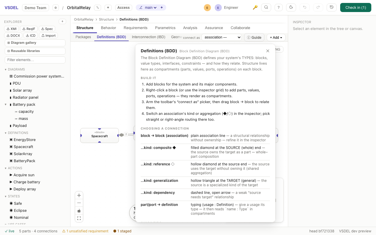
Named diagrams get the SysML frame with a corner tag; the PNG button exports the diagram — notation, frame and all — for review decks.
Keyboard shortcuts
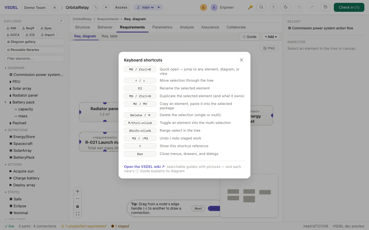
| ⌘K | quick-open anything |
| F2 | rename selection |
| ⌘D | duplicate (with owned children) |
| ⌘C/⌘V | copy / paste into the selected package |
| ⌘Z / ⇧⌘Z | undo / redo staged work |
| Delete | delete selection (single or multi) |
| ? | cheatsheet |
Import & export
In: No Magic/Cameo SysML v1 (.mdzip or XMI — the full v1→v2 conversion: package structure, blocks/interfaces/constraint blocks, value types and enums, parts with multiplicities, value properties with defaults, ports, generalizations, requirements with satisfy/derive/refine/trace, use cases and actors, activities with control flow, state machines with triggers and guards, and sequence diagrams (interactions with lifelines and messages) — re-import updates in place, and every import stores a conversion report: what each v1 construct became, what was skipped and why — and the XMI export writes the same coverage back for Cameo round-trips), ReqIF, DOCX requirement extraction, FMU co-simulation units, reusable definition libraries, and KiCad boards/netlists (.kicad_pcb/.net) into the Board lens. Out: XMI, ReqIF, generated specification documents (from any commit), diagram PNGs, ICD exports, KiCad .kicad_pcb/.net for routing, and a board BOM as CSV. Programmatic access via the OMG Systems Modeling API, an OSLC provider for DOORS/Jama/Polarion-class tools (bearer tokens minted in-app), and a stdlib-only Python client.
Self-hosting
VSDEL ships Dockerfiles, a compose file (including an optional MCP service), and a Helm chart for buyer-hosted installs. Self-host licensing uses signed keys; the MCP server runs beside your install with VSDEL_MCP_URL pointed at it, so agent tokens never leave your network.
Teams, roles & presence
Teams own projects; members hold per-project read / write / admin roles, and team admins manage every project in the team (Access button, top bar). Live presence shows who's working where; staged changesets are per-user so nobody tramples anybody; element locks are there when you want hard reservation. Invite teammates with an invite code from Team settings.
The fidelity ladder
Systems engineering starts at low fidelity and grows toward higher-fidelity models — CAD geometry, structural (FEA), thermal, behavioral. VSDEL keeps that a connected thread: any element can declare higher-fidelity realizations that stay linked to it and version with it. Select an element and open the Fidelity ladder in the inspector to add one.
- Declare a realization: pick a kind (CAD geometry, FEA, thermal, electrical, mission scenario, behavioral/FMU, physical prototype), set its maturity (concept → preliminary → detailed → released), and link the artifact (a STEP file, external CAD, a document, or an internal model element).
- Change capture across fidelity: edit the abstract element and its realizations are flagged suspect — the same mechanism requirement trace links use — so drift between the systems model and the high-fidelity model is never silent. Re-sync clears the flag.
- One spine, every domain: CAD is only the first kind; FEA, thermal, and behavioral realizations plug in identically. This is the bridge that lets fidelity grow without losing traceability.
Instance administration
Above team admins sits the instance admin — the operator of the whole VSDEL instance, configured by email on the server (ADMIN_PRINCIPALS). When an instance admin signs in, an Admin button appears on the project-home screen, opening a three-tab panel:
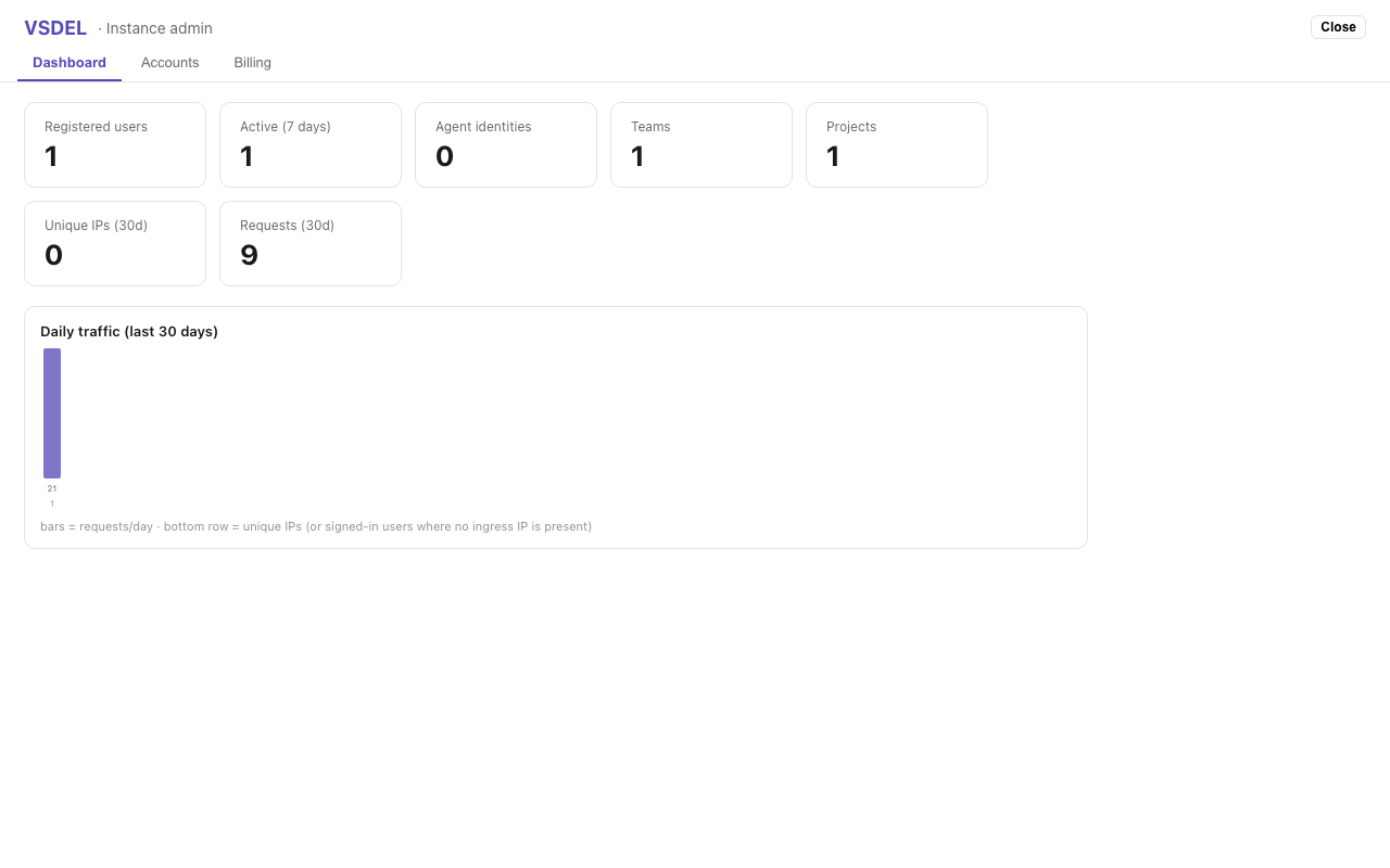
- Dashboard: registered users (with 7-day active count), teams, projects, unique visitor IPs and request volume over the last 30 days — collected by the server itself, no external analytics.
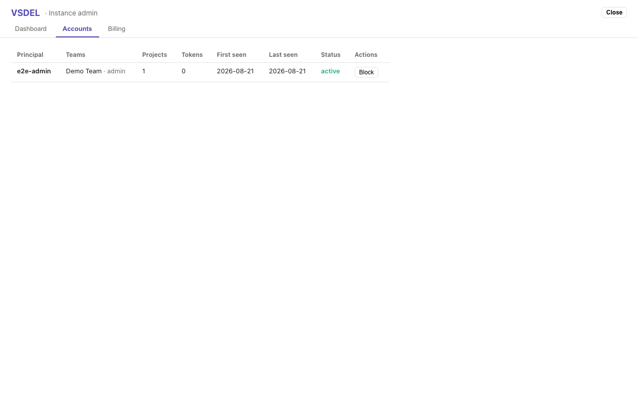
- Accounts: every principal that has signed in or holds membership — teams and roles, first/last seen, API tokens. Block disables an account instance-wide (sign-in still succeeds at the identity provider; every API call is refused until unblocked); Revoke tokens clears a principal's API tokens.
- 3D models: upload photorealistic
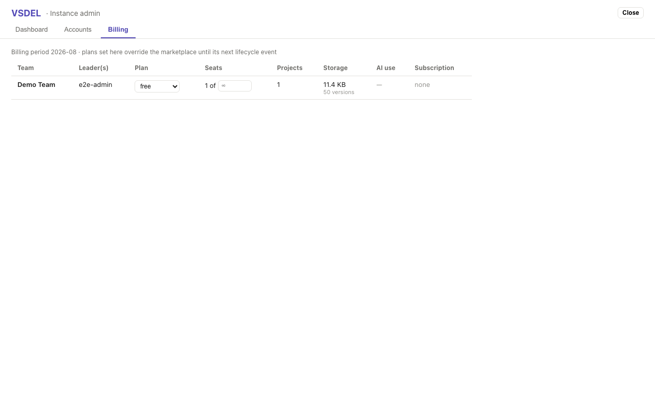
.glbmodels per element kind, served same-origin (no CDN) with automatic procedural fallback — see the mission lens. - Billing: every team with its leader(s) (team-admin members), plan (free / pro / enterprise), seats (members in use vs. purchased quantity, editable for direct deals and grants), project count, total storage (bytes of model data across the team's projects, committed + staged, with the element-version count), AI use (metered tokens this period and all-time), and the attached marketplace subscription. The plan dropdown overrides a team's plan directly; a paid plan with no subscription is badged manual grant — the mechanism for comps and gov/academic grants — and the marketplace webhook re-syncs subscribed teams on their next lifecycle event.
Plans & seats
VSDEL bills per seat: a team's seat count is its purchased subscription quantity, and the AI allowance scales with it. Team settings shows your seats in use and AI tokens consumed against the monthly allowance.
| Free | Pro — $49/seat/mo | Enterprise — $119/seat/mo | |
|---|---|---|---|
| Seats | 3 | as purchased | as purchased |
| Projects | 5 | Unlimited | Unlimited |
| Modeling (all views) | Full | Full | Full |
| AI assistant | — | 2M tokens/seat/mo | 10M tokens/seat/mo |
| Self-host license | — | — | Available |
When a team uses its included AI tokens for the month, the assistant pauses until the reset — add seats for a larger allowance. Government and academic teams can request a free Pro grant from the instance administrator (see Instance administration).
Milestones — lifecycle review gates
The Milestones lens tracks the program's lifecycle review gates — SRR, PDR, CDR, TRR and the rest — each with its date, status, and entry / exit criteria, so the schedule of formal reviews and the bar each one sets are captured with the model.
- The review gates: record each program milestone (SRR, PDR, CDR, TRR…).
- Dates & status: track when each gate is due and where it stands.
- Entry / exit criteria: state what must be true to enter a review and to pass it.
When to use it. Use Milestones to plan and monitor the formal review cadence of a systems-engineering program and to hold the criteria each gate must meet. It complements the model-level Reviews workflow — Milestones is the program's schedule of lifecycle gates, Reviews is the change-by-change approval of the model itself.
Reviews — propose, discuss, approve, merge
The Reviews lens is a model-review workflow: propose changes on a branch, discuss them, approve, and merge — a pull request for the model. Work is proposed against a branch, walked and commented on, and only merged into the mainline once it is approved.
- Propose on a branch: open a review over the changes staged on a branch rather than committing straight to the mainline.
- Discuss the diff: reviewers walk the proposed changes and comment.
- Approve & merge: once approved, the branch merges back, with conflict resolution where needed.
When to use it. Open a review whenever a change should be seen before it lands — a trade-study branch, a colleague's contribution, or a claimed set of AI-agent proposals. It builds on the tool's branch-and-versioning model, giving human sign-off on the model the way a code review does for source.
Slider, the AI assistant
Slider is the built-in AI helper (Collaborate pillar, paid plans), docked at the foot of the inspector — a little slide-rule that comes alive while it's working. It reads the live model through the same API as any client and can build model content on request, and every edit it proposes lands as a staged change in your working set, reviewed and checked in like any human edit. It streams its tool activity so you can watch what it reads and writes. Click Slider to open the full chat.
✨ Generate from text. Paste a specification paragraph (+ Add ▾ → Generate from text) and Slider extracts the model it implies — requirements with their shall-statements, the parts and attributes they mention, and the satisfy links connecting them — staged as one reviewable batch in your check-in drawer. Nothing commits until you check it in.
🔍 AI review. Before checking in, the drawer's AI review button has Slider read your staged set alongside the model's own health checks and validation rules, then report findings ordered by severity — grounded in the actual checks, flagging problems rather than silently rewriting your work.
Bring your own AI. Prefer to run Slider on your own model? Click the provider chip on Slider and choose a provider — Anthropic, OpenAI, Azure OpenAI, or any OpenAI-compatible endpoint (Ollama, vLLM, OpenRouter, LM Studio) — then enter your key and model. Slider keeps the same knowledge of your model; only the AI engine changes. Requests run on your own account and bill, so the plan's monthly AI allowance doesn't apply. Your key is stored only in your browser and sent to VSDEL only to run your requests — never saved on our servers. The model must support tool calling. Self-hosters pointing at a local model (e.g. Ollama on localhost) enable it with VSDEL_ALLOW_LOCAL_AI=1.
External AI agents (MCP)
A team admin can authorize an outside agent — Claude Code, Claude Desktop, or any MCP client — to model in the team's projects. Mint a token in Team settings → AI AGENTS (shown once; revocable), point the client at the hosted MCP endpoint, and the agent can read models and topology, stage elements/relationships/diagrams/layouts/deletes, and arrange drill-down decompositions — all as proposals under its own identity. It cannot check in, merge, or administer anything; the server enforces that for every agent credential.
Agent proposals appear under the 🤖 badge in your check-in drawer — Claim into my changes adopts them (with "proposed by" provenance; anything skipped is reported, never silently dropped), then you check in as yourself. The bundled vsdel-modeling skill teaches agents the SysML vocabulary and the house conventions, so their output arrives claim-ready.